Reducing Local QRM With A Few Ferrite Cores

One downside to an SDR is that you more easily notice the mysterious carriers and other local noise/RFI signals. After reading this article on Common Mode Chokes, I decided to see what I could do to improve my situation.

As a first step, I captured this baseline of the 6500-7000 kHz range, where I am most interested in listening (click to enlarge):

I then added a choke on the antenna input to the SDR, right where it enters the radio. It is 9 turns of the coax on a large toroid core, probably type 37 or 43 material, possibly a Fair-rite 5943003801:

The other coax cable next to the antenna input is the reference signal from the 10 MHz GPS reference. Adding ferrite to it had no effect. I’ll get to the orange toroid next. Here is the result (click to enlarge):

As you can see, there was a significant reduction in the number of carriers and other noise signals.

Next I added the orange toroid also pictured (unfortunately I have no idea what type of ferrite it was, it was from the junkbox), as well as two of the clamp on ferrites you often see on AC power or video cables to the ethernet cable that runs from the SDR to the computer, here are the results: (click to enlarge):

This got rid of a few more. Pretty much, what is left is an actual signal. I was able to identify these:
6604 New York Radio
6519 A voice transmission, perhaps another VOLMET
6660 The second harmonic of CHU 3330
6725 An RTTY transmission
6885 Israel fading in
6970 faded in and out, so it seemed to be a legit DX station

Here’s a slightly later shot of 43 meters (6800-7000kHz):

All in all, a significant improvement, for a few minutes worth of work!

6914 kHz Mystery Station

This weekend, I’ve noticed a station transmitting periodically on 6914 kHz. It will come on the air for a few minutes, then go off. All transmissions appear to be AM, with a variety of modes, such as CW (so MCW in this case), RTTY, and even some voice.

Last night I heard transmissions until the last one ended at 0136 UTC, when they stopped until 0745 UTC this morning. None were noted on the SDR recording during that time period.

When the transmissions restarted at 0745 UTC, they were extremely weak.

Here is an RTTY transmission (again, sent in AM mode) using 1000 Hz shift, 45 baud, with a center frequency of 1700 Hz, received at 2345 UTC 1 June 2013:

AGA5D2 DE A39P. FROM XXX DEFPAT ECHO X2 RTB XXXAFTER ACTION K
ART KKDUQLGLZXPQORU TUYI YUUOI PIOIU OUIYY WETYU IYOUI QRWET YTUII IUOPQ WYTUR TIOOQ PPOUY YYIER WEITY URYYU WQPOP TWLA IPQUQ QITWI PUPUQ IYUYR EWPQU TUIOW O
JAL4-6756 38677 192864 BT

A39P DE A5D2. ROGER OUT

The signal was not the best, so there are some errors in the decoded text. Here is an Audio recording of the transmission.

Here is a CW transmission at 1358 UTC on 2 June 2013:
And the decoded text, thanks to Token for providing it:
AHDR DE A50S COME IN K
A50S DE AHDR RGR GO AHEAD K
AHDR DE A50S CONTINUING ON SECPAT ROUTE. ALL CONDITIONS NORMAL K
A50S DE AHDR RGR COPY ALL K

Here is a voice transmission at 1431 UTC on 2 June 2013:

Token has reported this station on both 6914 and 23146.5 kHz back in December 2012.

Homeopathic Radio Engineering

Mainstream radio engineering principles hold that the received signal strength of a transmission is proportional to the radiated power. Doubling the transmitter power produces twice the received power, quadrupling the transmitter power produces four times the received power, twice the received voltage, which is 6 dB or one S unit. This has been accepted for over a century.

However, recent experimental results, first reported on the FRN and later in The Journal of Irreproducible Results cast doubt in this basic radio engineering theory.

These results claim that as the transmitter power is reduced to very low levels, the received signal strength actually goes up, not down.

A transmitter location on the east coast of the USA was used. The tests were conducted on HF radio frequencies on and around 6925 kHz, using a state of the art solid state transmitter with a standard off the shelf MOSFET as the RF final amp:

Each monitoring post was equipped with the highest quality HF receiving gear and highly sensitive monopole receiving antennas.

During the trials, it was found that placing a non-conductive fabric, such as a sock, over the receiver produced the strongest signals. While the exact mechanism for this effect is not yet known, it is presumed to be due to the high dielectric constant of the fabric.

The results of the experiment clearly speak for themselves, as transmitter power went down, the signal strength went up:

One way to explain the results is to return to the luminiferous ether theory of radio propagation. Radio waves are propagated by vibrations in the ether. Fewer radio waves means that there is more ether per radio wave, so the vibrations are larger, producing a stronger signal at the receiving site.

There were even reports of radio propagation that cannot be explained by any known laws of physics, such as signals in the daytime traversing from Montana to New Zealand on 6955 khz with a completely sunlit path, even though D layer absorption would make this completely impossible. Yet this was reported many times by longtime radio physicist Dr. Winston: “The signals were always received with as SIO of 555. Even the audio quality was perfect, why it sounded like I was listening to it live in the studio!”.

Several times signals were actually received and logged on the FRN before the transmission began. This suggests that superluminal neutrinos may be involved.

Further research into this new phenomena is required. If homeopathic radio is ever perfected, it would allow listeners to report hearing transmissions that used little, or theoretically even no power. Indeed, reducing the output power to zero watts might produce the best results of all for this type of station.

WWV and WWVH Via Both Long and Short Path on 15 MHz and I can Hear Russia From My House

In Measuring The Distance To A Shortwave Radio Station we looked at how the propagation delay in a shortwave signal can be used to estimate the distance to the station.

I ran some more tests the other day:

Below is a recording of 15 MHz, taken at 2300 UTC on December 13, 2012:

The GPS 1 PPS reference is on the top trace, and the audio from the radio is on the lower trace.

You can see the one second tick pulse from WWV in the audio, as well as two pulses from WWVH, the first (weaker) one is the normal (short) path signal, and the second one is via long path. We can confirm this is the case by converting the time delays into distance. We’ll use the same formula as in the previous article, we subtract off the 286 sample delay from the radio, multiply by 22.676 to convert the delay in samples to microseconds, then multiply by 0.186282 (the speed of light in miles per millisecond) to convert the delay into miles.

For WWV, the measured delay from the 1 PPS pulse is 660 samples. (660-286) * 22.676 * 0.186282 = 1580 miles
For WWVH short path, the measured delay was 1516 samples: (1516-286) * 22.676 * 0.186282 = 5196 miles
For WWVH long path, the measured delay was 5080 samples: (5080-286) * 22.676 * 0.186282 = 20250 miles

The distance to WWV is 1480 miles, and to WWVH is 4743. The long path distance to WWVH is 20158 miles.

Remember, the calculated distances can be longer than the great circle distance, due to the signal making one or more (many more in the case of long path) hops between the Earth and the ionosphere. Plus, there is the experimental error.

And here is one more example, this time it is the Russian time station RMW, on 14996 kHz, recorded at 1157 UTC on December 10, 2012:

The delay was 1835 samples: (1835-286) * 22.676 * 0.186282 = 6543 miles.
The great circle distance is 4821 miles.

Measuring The Distance To A Shortwave Radio Station

In a previous post, I showed how it was possible to crudely measure the speed of light (or at least another type of electromagnetic radiation, radio waves, in this case) by measuring the time delay between two shortwave radio time stations, WWV and WWVH.

I’ve decided to re-do that experiment, but in a slightly different way. Rather than measure the speed of propagation, I will use that speed to determine the distance to the radio station.

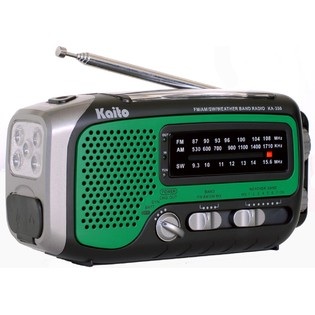
Various time stations transmit precise time on several shortwave frequencies. Here in the USA, we have WWV in Ft. Collins, Colorado, which transmits on 2.5, 5, 10, 15, and 20 MHz. We also have WWVH in Kekaha, Hawaii, which transmits on 2.5, 5, 10, and 15 MHz. These stations transmit an audio “tick” at exactly each UTC second. There is also the Canadian station CHU, located near Ottawa, Ontario, which transmits on 3330, 7850, and 14670 kHz.

One way to measure the speed of radio waves (and light) would be to measure how long it takes for the tick to travel a fixed distance. Divide the distance by the time, and we have the speed of light. However, that requires knowing the exact UTC time locally. This can be done with a GPS unit that outputs a 1 PPS (pulse per second) signal.

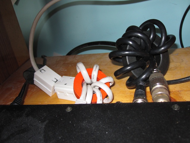
How to feed these signals into the computer, so they can be measured? The radio audio is easy enough, feed it into the sound card. It turns out the 1 PPS signal can also be fed into the sound card, on the other channel. I used a capacitor to couple it.

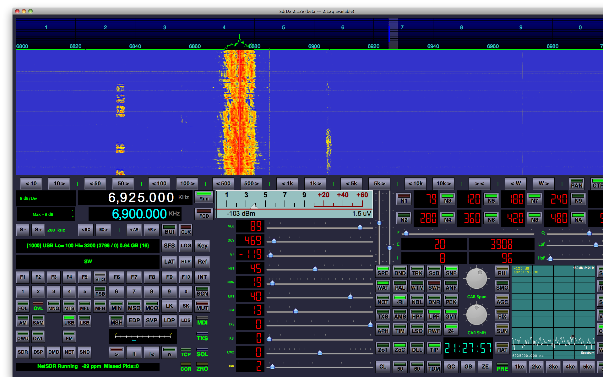
The first measurement that is required is one to determine what time delay is added by the radio electronics. In my case, I was using a JRC NRD 545 receiver, which has DSP (Digital Signal Processing) to implement the audio filters. This certainly adds a time delay. I therefore needed to run some baseline measurements, to determine how long this delay was.

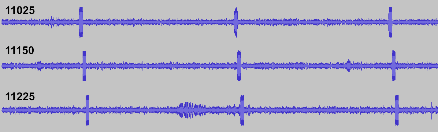
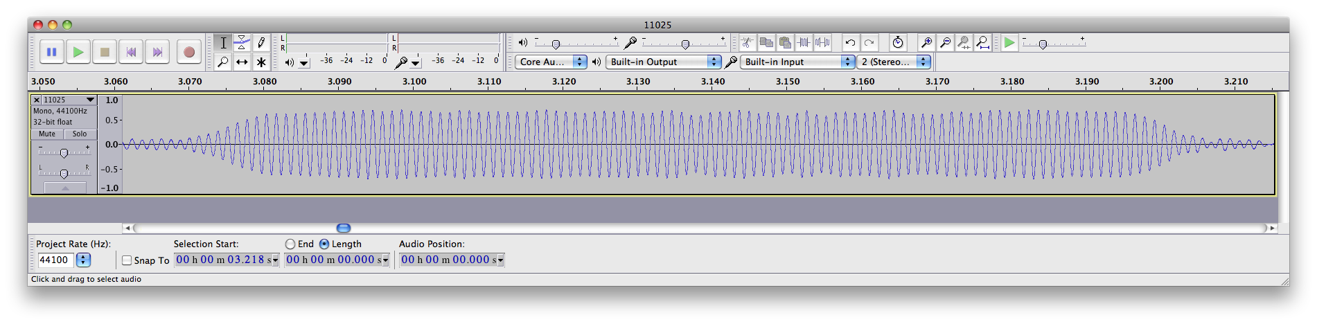
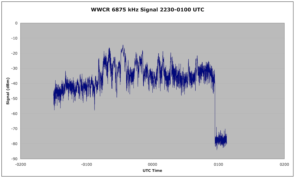
I fed the same 1 PPS signal into the antenna jack of the radio. The signal is a short (10 microsecond pulse) that is rich in harmonics, so it produces a noticeable “tick” sound every second. I then recorded the audio from the radio, along with the 1 PPS signal fed into the other channel, and obtained this data (click on the graph to enlarge it):

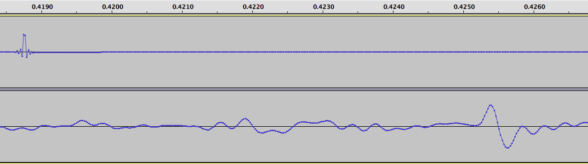
I measured the time delay between the two ticks, and found it to be 286 samples. At 44.1 kHz, each sound sample is 22.676 microseconds. Multiplication gives us the time delay, namely 6485 microseconds. This delay added by the radio is constant, provided I do not adjust the IF filtering parameters (which were set to USB mode, 4.0 kHz wide, for all tests).

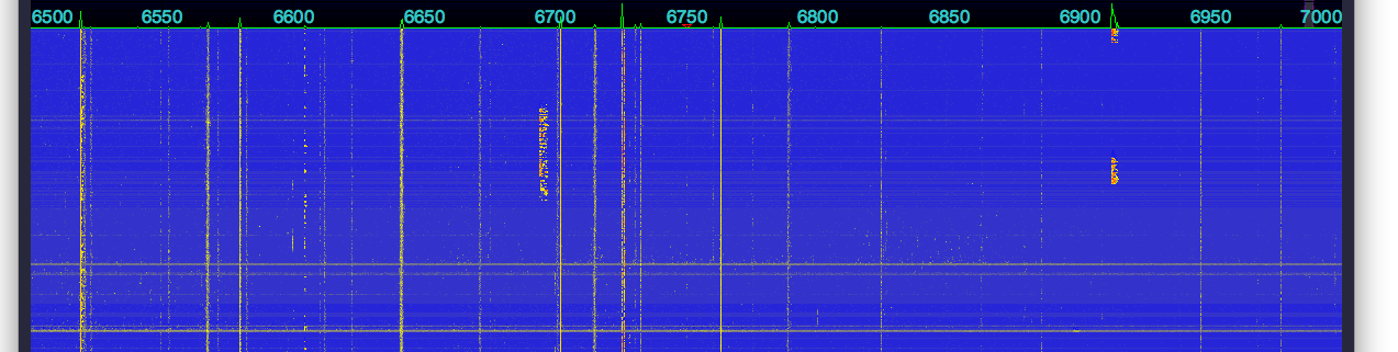
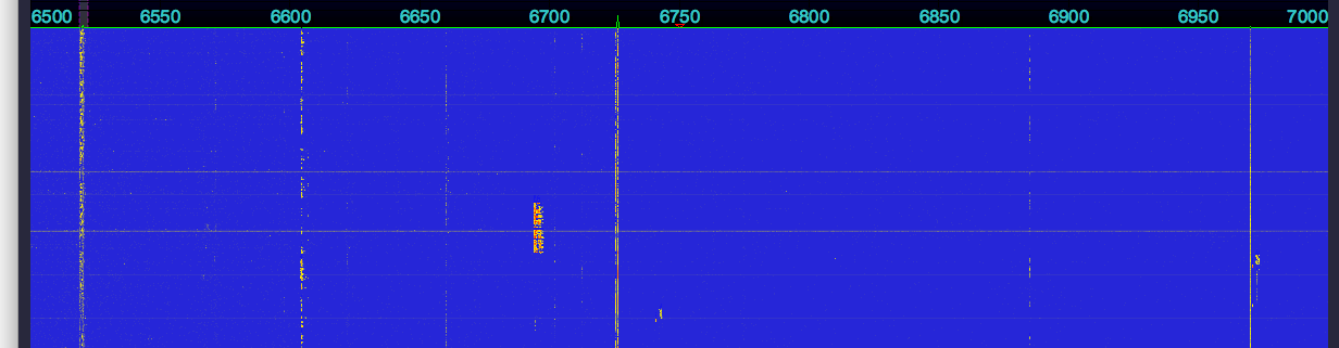
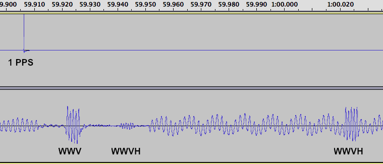
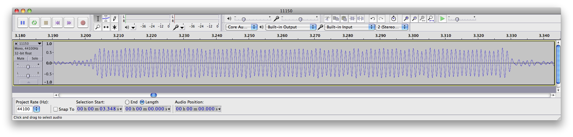
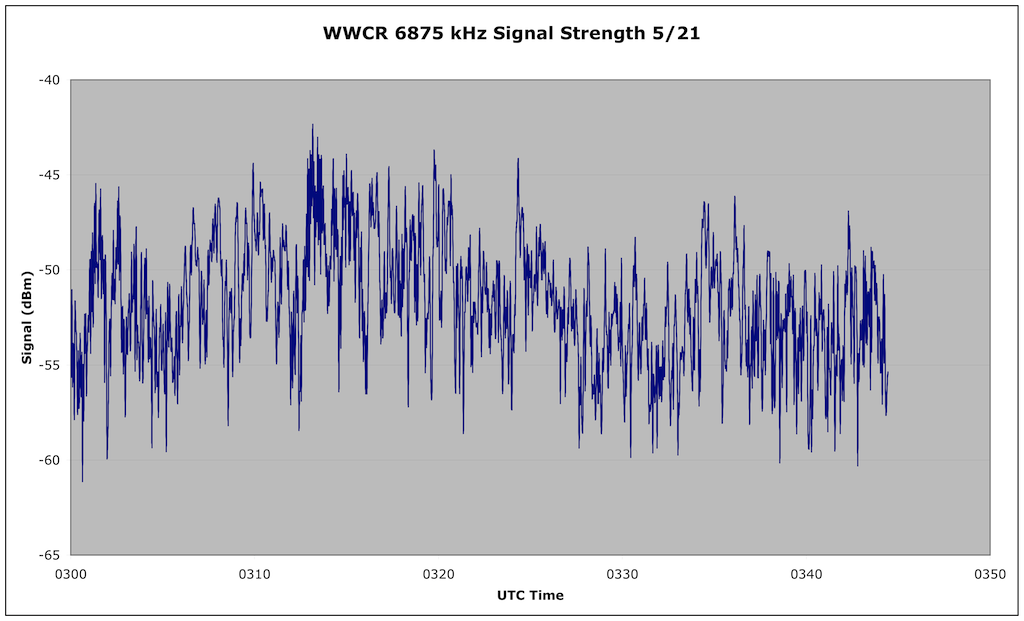
Next, the antenna was reconnected, an the radio tuned to 15 MHz. At this time of the day (about 2100 UTC) it is possible to hear both WWV and WWVH. Here’s the sound recording:

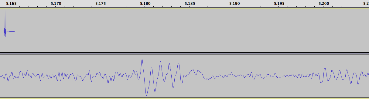
The WWV pulse occurs at about 5.18 seconds on the recording, and WWVH, much weaker and harder to see, at about 5.2 seconds.

The delay for the WWV pulse is 657 samples. Subtracting the radio delay of 286 gives us a delay due to propagation of 371 samples. Multiplying by our conversion factor of 22.676 microseconds per sample gives us 8413 microseconds.

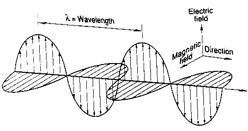
Light (and radio waves) travel at 186,282 miles per second or about 0.186 miles per microsecond. For the metric inclined, that’s 299.792 km/sec or 0.300 km per microsecond. So multiplying our time in microseconds by the distance light travels each microsecond gives us the distance:

8413 * 0.186 = 1567 miles (2522 km)

The actual distance, along the Earth’s surface, from my location to WWV is 1480 miles, or 2382 km. Why the discrepancy? The radio waves do not travel along the Earth’s surface, but instead are reflected from the ionosphere, which is several hundred miles up. This means the actual path they take is longer. We’ll try to take that into account, a little further down.

The delay for the WWVH pulse is 1550 samples. Subtracting the radio delay of 286 gives us a delay due to propagation of 1264 samples. Multiplying by our conversion factor of 22.676 microseconds per sample gives us 28662 microseconds. We’ll do our next multiplication again, to convert to distance:

28662 * 0.186 = 5339 miles (8592 km)

The actual distance from my location to WWVH is 4743 miles, or 7633 km.

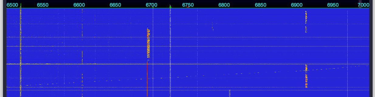
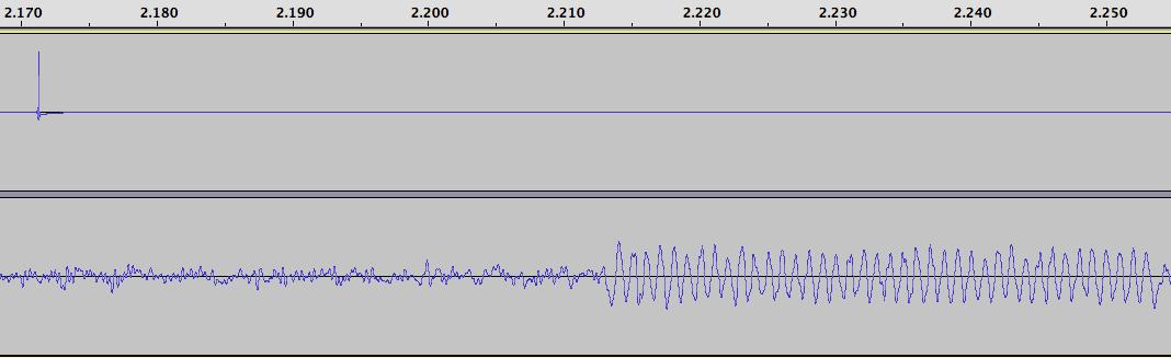
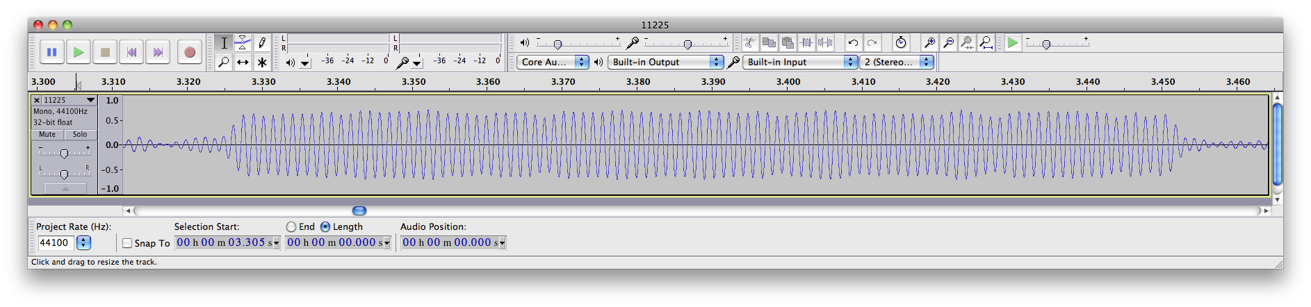
Next, here’s a recording from the Canadian time station, CHU:

The delay for the CHU pulse is 401 samples. Subtracting the radio delay of 286 gives us a delay due to propagation of 115 samples. Multiplying by our conversion factor of 22.676 microseconds per sample gives us 2607 microseconds. We’ll do our next multiplication again, to convert to distance:

2607 * 0.186 = 486 miles (782 km)

The actual distance from my location to CHU is 407 miles, or 656 km.

Now let’s try to take into account the actual path of the radio waves, which get reflected off the ionosphere. We need to know the height of the ionosphere, which unfortunately is not constant, nor is it the same over each part of the Earth. Here is a map showing the approximate height, while the above recordings were taken:

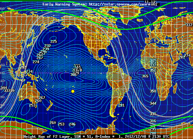
In the case of the path to CHU, the height is about 267 km, or 166 miles.

We also need to determine the straight line path between my location and CHU, through the Earth, vs the distance along the Earth’s surface. This can be calculated, and it is 391 miles, or 629 km.

We’ll determine what the actual path length is for a radio signal traveling this distance. It looks like a triangle, with a height of 166 miles, and a base of 391 miles. We need to determine the other two sides to find the total path length. All we need to do is take half of 391 miles, which is 195.5 miles, square it, add to that 166 squared, and take the square root, then double our answer. The result is 513 miles, which is very close to our measured value of 486 miles. We’re off by a little more than 5%.

Next let’s try WWV: The actual distance is 1468 miles or 2362 km. Doing our math, using an approximate FoF2 ionosphere height of 246 km (153 miles): Half of 1468 miles is 734 miles, we square that and add to 153 squared, and take the square root, and double our answer, getting 1500 miles. Our measured distance was 1567 miles, so we’re off by less than 5%.

Next, the case of WWVH. This is more complicated, as the signal probably is making more than one “hop”, that is, it is going up to the ionosphere, reflected down to Earth, and then reflected back up again, and down again. This may possibly occur multiple times.

We’ll try doing the math anyway. The actual distance is 4588 miles or 7383 km. Doing our math, using an approximate FoF2 ionosphere height of 253 km (157 miles): Half of 4588 miles is 2294 miles, we square that and add to 157 squared, and take the square root, and double our answer, getting 4598 miles. Our measured distance was 5339 miles, an error of 16%. But again, we don’t know how many hops there were. Still, not a bad effort.

Does anyone else have a GPS receiver with a 1 PPS output? If so, I’d like to hear from you, I have some additional experiments in mind.

Mysterious Ditter Network

First observed two days ago, there seems to be a new (to us HF listeners, anyway) network of HF ditter CW transmissions. The purpose of this network, as well as who is operating it, is unknown. It is possible they are for propagation monitoring. Based on observations of listeners and propagation characteristics, it would appear that at least some of the transmissions are coming from North America, possibly the Central US.

The transmissions do not occur at the same time on all frequencies. It appears that each transmitter steps through the frequencies. The following image shows the received signal on three of the frequencies (click on the image to view it as a larger size):

As you can see, thea transmission on each frequency begins right after the transmission on the previous frequency ends. This data was obtained by running a netSDR receiver in 500 kHz wide I/Q capture mode. The resulting recording file was then demodulated at each frequency of interest.

You can also see the second (weaker) dit on the 11150 tranmsission, that occurs shortly before the stronger main dit. (It is less obvious before the second dit, but you can see it, if you squint)

Each pulse (dit) is 130 milliseconds long, and they repeat every 6 seconds.

Next, the demodulated signal for a ditter transmission on each of the above frequencies is shown magnified, to see the exact times of each transmission.


How to find these transmissions:

I find that using an SDR is the easiest way, as you can observe a large portion of the spectrum at once. I use a 500 kHz wide view, and step through HF, looking for the periodic dits. But you can certainly use any radio. Note that the frequencies are all multiples of 25 kHz. They also sometimes occur in groups of three relatively associated frequencies. There are likely additional frequencies that have not yet been discovered.

If you’re hearing any of these transmissions, or have discovered possible additional frequencies, please let us know with a comment!

Transmissions on the following frequencies have been observed (all in kHz):
5450
5575
6225
6550
6750
7700
8000
8275
8775
8825
8900
8975
9050
9225
10050
10450
10575
10900
11025
11150
11225
11300
12450
13100
13250
13325
13875
14400
15100
15400
15625
16000
16350
16550
16725
17475
17650
17950
17975
18050
18100
18200
18450
18625
19300
19650
20100
20175
20250
22050
24050

Building a Sky Loop Antenna

Due to the continuing interest in the sky loop antenna, I’ve put together some notes and suggestions on the construction of these incredibly well performing antennas. One note – the sky loop is generally used as a receiving antenna. I don’t have any first hand experience using one for transmitting. Typically, the SWR is all over the place, so you’d likely need a tuner if you wanted to transmit with one. For receiving, no tuner is needed. The sky loop covers all of HF, and often down into MW as well, depending on the size.

First, the basics. A sky loop antenna is a large loop of wire mounted in the horizontal plane. How large? Typically, as large as you can make it. Bigger is generally better when it comes to sky loop antennas. Mine has a perimeter of 670 feet, and I am considering enlarging it. Often, this antenna is run around the property line of your yard, maximizing the length of the antenna as well as the cross sectional area. While the antenna is called a loop, this does not imply that it needs to be circular in shape. While a circle does maximize the area for a given length of wire, other shapes work well. Remember, you’re trying to maximize the amount of wire (perimeter of the loop shape) and area, so try to use as much of your yard as possible, although you don’t want to zip zag back and forth too much. You want to make the largest area polygon that you can. The likely constraint will be what trees or other supports you have available for getting the wire in the air. And of course, remember that safety is important – keep the wire far away from any overhead power lines.

Because the antenna is in the form of a loop (a continuous path of wire from one of the transmission line terminals to the other), it is inherently a low noise antenna. Comparing a sky loop to a dipole, you will find that the noise levels are generally much lower.

How to get the wire in the air? There’s lots of ways, what I find that works best is to put rope up into trees around the path I want the antenna wire to run. One end of the rope has an antenna insulator, the rope then goes up over the tree (or a branch or whatever you can manage) and the other end is secured to keep the insulator up in the air. I just put a large nail in the tree, pull the rope taut, and then wrap it around the nail several times to secure it. often I will put a second nail in the tree as well, a few feet below the first, and then coil the excess rope around the two nails, to keep it neat and tidy, and away from rope eating lawn mowers. Untying rope that’s been wrapped around mower blades is no fun. Been there, done that.

I use an EZ Hang to put rope up in trees.

The antenna wire itself then runs through the other end of the insulator. Since the wire is in a loop, this requires some planning, you need to put a bunch of insulators on the antenna wire, as many as you will need, and then use one for each of your antenna support ropes.

Here’s how I do it:

The EZ Hang shoots a fishing weight up and over the tree. There’s fishing line attached to the weight. Once the weight lands on the other side of the tree, I take off the weight, and attach the end of the rope to the fishing line. Then I use the reel on the EZ-Hang to pull the rope back through the tree, until it gets down to the ground at the EZ-Hang. Now I’ve got the rope going up and over the tree and back down. Then I can cut the rope off the spool, and attach an insulator (with the antenna wire already running through the other eye) to one end of the rope, and pull it and the antenna wire up into the air.

If your antenna is relatively small, you may get away with just four or so insulators, one at each corner of the loop. As the antenna gets larger, you end up with a lot of sagging due to the weight of the wire, and you need several intermediate support insulators on each side of the loop, to limit the sagging.

As far as the type of wire to use, there’s several possibilities. First, of course, is normal stranded copper antenna wire. I, however, got a great deal on a 1000 ft spool of #16 insulated wire. I went with that because the antenna wire would be going through trees and leaves, and wanted to minimize the chances of the wire being shorted out to ground. While probably not as important with a receiving antenna like this as with a transmitting antenna, I decided to play it safe. Also, the insulation happens to be green, and I think it does a good job of helping the wire to blend in the trees, making it difficult to see.

There’s a lot of debate as to how high the wire for a sky loop antenna needs to be. Computer modeling shows that the higher it is, the better it is at picking up low angle signals from DX stations. And in general with HF antennas, higher is better. On the other hand, if it is difficult for you to get the wire up very high, a sky loop with low height wire is still going to perform better than no sky loop at all. I started out with several sides of my sky loop being relatively low, 15 ft up or so, because that is what I could easily manage. Then, over time, I have raised those sections as I was able to. I do think the antenna performs better now that it is higher up, but I am not sure that the effects are dramatic. So my rule of thumb would be to get the wire up as high as practical, but I don’t believe there is any magical height you must achieve. Right now, the height varies between about 25 to 50 feet.

As I mentioned at the beginning of this article, the SWR (and feedpoint impedance) of a large sky loop antenna is all over the place. If you think about it, for many SW bands, the antenna is several wavelengths long. In my case, the antenna is about 670 (206 meters) feet in perimeter. So for the 43 meter pirate band (say 6.925 kHz), it is about 4.75 wavelengths long. At 15 MHz, it is over 10 wavelengths long. That said, I do not use an antenna tuner. While you could, I don’t think it is necessary for receiving applications. The antenna collects lots of signal, and I don’t believe you need to squeeze out the last S unit.

Since the impedance is usually quite high at any given frequency, I chose to feed the sky loop antenna with a 12:1 balun. I didn’t choose this based on any calculations, I just happened to have one available. I do keep meaning to try swapping other baluns, such as a 4:1 or even a 9:1, to see if there is any difference in the performance, but I have not gotten around to it. I do think some sort of balun is desired for the sky loop antenna, vs feeding it directly with just coax. You may be able to feed it with ladder line, but I have not tried that.

For the coax, I used RG6, which is commonly available and used for TV. I chose RG6 because it is very cheap, and personally I am sick of putting PL-259 connectors on coax. RG6 has F connectors, and I use an F to PL-259 adapter at the balun, as well as to connect to the radio inside the shack. There’s certainly no requirement to use RG6, you can use any good quality coax.

Performance does suffer once I get down to about the middle of the Medium Wave band. While I can pick up stations all the way down to 530 kHz, the signal strengths are much less than the upper end of the medium wave band. If you assume the antenna is a basic loop, the resonant frequency is about 1460 kHz, so this seems reasonable. I get excellent reception in the X band, 1600-1710 kHz. One of my reasons for wanting to increase the length of the loop is to hopefully get better performance lower down in the MW band. Although simple math shows that even if I doubled the length (which I am not sure I could do), the resonant frequency would still only be about 730 kHz.

Another possibility for worse performance on the lower part of the MW band is the choice of balun, as I addressed above. The impedance of a one wavelength loop antenna is about 120 ohms. With a 12:1 balun, that is reduced to about 10 ohms. And at the lower end of the MW band, the impedance is likely much lower.

If you’ve read my This is why you should disconnect your antenna during a storm article, you’ve seen what happens when you have a thunderstorm nearby. Your antenna is often quite good at collecting that energy, and sending it to your radio. There’s lots of good lightning protection devices out there that you may want to look into. Personally I also disconnect my antenna when there’s a storm, or even the possibility of a storm, especially if I am not going to be around. It takes a few seconds, and can protect your radio. It doesn’t take a direct lightning strike to damage a radio.

I hope this article will motivate several listeners who have the room to consider installing a sky loop antenna. You won’t be disappointed.

Vladimir Putin Destroys Pirate Radio

For the last few weeks, there’s been a new source of QRM on the most popular shortwave pirate radio frequency in North America, 6925 kHz. Last night, it was particularly bad. Here’s a recording of what it sounds like, when tuned to 6923 khz USB.

Putin on the QRM

The offending signal is a Russian Military 12 Tone PSK AT-3004D modem, often referred to as the “Russian 12 Tone Modem” in utility DXer circles, and also the MS5.

There is a very good writeup about it at this site: http://www.signals.taunus.de/FFT/CIS12CH.HTML

Here is an SDR waterfall image of the modem:

You can see the stronger pilot carrier on the extreme right (highest frequency) as well as the 12 PSK channels.

The signal faded in at around 2300 UTC, was quite strong around 0030 to 0200 UTC, and faded out around 0400 UTC. The local fade in time is due to the Sun starting to set here, and the path being mostly dark, to support propagation on this frequency. The fade out time is due to sunrise at the transmitter site. This suggests a location somewhere in Europe.

If this modem continues to transmit around 6925 kHz, operators may wish to work around it, by avoiding 6925 kHz during the time the 2300-0400 UTC time the signal is present. Unfortunately this is also the most popular time for pirate transmissions. Due to the strong signal strength, and the wideband nature of the signal, it can to obliterate any weaker stations on the frequency.

Daytime Vs Nighttime Static Levels And The Impact On Reception

Undercover Radio was on 6925 kHz USB several times on Sunday, May 20, 2012, conducting some transmitter tests in the afternoon, and with a show in the evening. I noticed how, even with a relatively weak signal strength in the afternoon, the overall reception was still good, due to the low daytime noise levels on the 43 meter band. Transmitter power was around 20-30 watts PEP.

Here is a graph showing the signal level of Undercover Radio on 6925 kHz, as well as background noise from an otherwise unoccupied adjacent frequency for 4 minutes, starting at 1700 UTC May 20, 2012:

Undercover Radio’s signal strength was about -92 dBm. Bear in mind that this was a voice only program with Dr. Benway talking, with frequent pauses in speech. Since this was an SSB transmission, the received signal level falls to the background noise level during pauses in speech.

The background static at 6930 kHz was -100 dBm

The net result is a signal to noise ratio of 8 dB, which is certainly adequate for fair to good reception.

Some recordings:
Undercover Radio 6925 kHz USB 1700 UTC
Background noise 6930 kHz USB 1700 UTC

Undercover Radio came back on at around 1900 UTC. Here is another comparison of Undercover’s signal vs background noise on 6932 kHz:

(Sorry, this time the noise is pink and the signal is blue. Just to keep you on your toes)

Eyeballing the graphs, it looks like the signal to noise ratio was about 15 dB, better than before. The quality of the received audio was indeed very good. Here is a recording

Next, Undercover Radio came on again at 0212 UTC.

The noise levels were around -85 dBm. Undercover Radio’s signal started at just around the noise level. At the time, he was running 20-30 watts PEP. Later, around 0245, Dr Benway realized he didn’t have the amp on, and then switched it on, going to 500-600 watts PEP.

One reason for the much higher nighttime noise levels is that not only is 43 meters open to DX from distant stations, but also to distant thunderstorms and other noise sources. Think of every thunderstorm in the world as a transmitter (which it really is). There’s thousands of active thunderstorms at any time, transmitting RF energy over the entire radio spectrum. This energy is received at your location from whatever parts of the world propagation is open to, on a given frequency. So while your signal can get out further at nighttime, it also has to compete with a lot more QRM sources.

During the daytime, the D layer of the ionosphere attenuates low angle radiation on 43 meters, preventing DX reception. You’re limited to just a few hundred miles. This applies both to the signals from radio stations that we want to hear, and distant noise sources.

Also notice how much Undercover Radio’s signal varied after the amp was switched on – by around 30 dB. That’s five S units! This tells us that signal reports, or even recordings, can be very hit or miss. One minute, an op can be at the noise level, a few minutes later, he can be many S units above it.

Two recordings. First, one from 0222 UTC when he was running 20-30 watts PEP, and the SNR was just a few dB. And second, one from 0300 UTC during a signal peak, when he was running 500-600 watts PEP, and the SNR was about 25 dB.

For comparison, here are some plots of WWCR, 6875 kHz, showing their signal level last night:

First, from 2230 to 0100 UTC (sorry for the X axis scaling, showing -100 for 2300 UTC. Blame Excel)

You can see that when their carrier went off the air, the noise level was around -80 dBm. And the signal varies by about 30 dB during the transmission, during nighttime. Earlier in the transmission, while it was still daytime, the signal was slightly weaker, but there was a lot less fading.

And second at 0300 UTC:

Perhaps the main point to take away from this is that while a pirate can be heard much further at nighttime than during the daytime on 43 meters, the lower noise levels and lack of significant fading during the daytime generally make for better quality reception, for those listeners within the several hundred mile NVIS range, and allows reception by listeners with more modest receiver/antenna setups. This is especially true when using lower power (grenade type) transmitters. Nighttime DX reception quality will be poorer, and limited to those with more substantial receiving stations. By selecting the time of day for operation, operators can to some degree select their audience and target area. A pair of transmissions, one in the daytime and one at night, would reach both local and DX listeners.

She had your dark suit in greasy wash water all year

An unidentified station was first noted at around 0330 UTC May 17, 2012, on 6990 kHz, sending three phrases over and over:

“She had your dark suit in greasy wash water all year. Don’t ask me to carry an oily rag like that. They used an aggressive policeman to flag thoughtless motorists”

I made this recording on 6990 kHz USB at 0041 UTC on May 17, 2012:

As of 2315 UTC on May 17, 2012, the station has moved to 6950 kHz USB, with the same repeated phrases.

Andrew Yoder reports hearing this same station on November 5, 2011 on 21450.7 kHz.

Some quick searches of the internet came up with something called the TIMIT Sentence Prompts.

According to Wikipedia:

TIMIT was designed to further acoustic-phonetic knowledge and automatic speech recognition systems. It was commissioned by DARPA and worked on by many sites, including Texas Instruments (TI) and Massachusetts Institute of Technology (MIT), hence the corpus’ name.

TIMIT consists of phrases of 630 speakers of of different sexes and eight major dialects of American English. The database is designed to assist in the development and testing of Automatic Speech Recognition systems.

There is an online listing of the phrases. According to that list, phrases 1, 2, and 437 are being sent.

Presumably someone is testing a system to perform automatic speech recognition on HF transmissions, and is conducting some real world test.

There is a thread of loggings of this station over at the HFUnderground Message Board.

I can only hope they don’t accidentally start transcribing 6925 kHz while Toynbee Radio is on the air. That could cause their computer to blow up, a la Kirk’s ability to make computers self destruct by confounding them with illogic on Star Trek.

Some online references:
The DARPA TIMIT Speech Database for MastersThesis
The DARPA TIMIT Acoustic-Phonetic Continuous Speech Corpus

UPDATE:
Still going at 1128 UTC on 6950 USB.