Atoms To Go     
   Periodic Table of the Elements for iPhone/iPad/iPod     

While shortwave radio is commonly thought of as being used for long distance communications, it also functions for local and medium distance links. This is accomplished by a method known as NVIS, or Near Vertical Incident Sky Wave, and is in fact what most US pirate operators are using, even if they have never heard of it before.

I touched on NVIS in my previous post Going Long, which readers may wish to read before continuing.

To summarize, the ability of HF radio waves to get from the transmitter to target location depends on the ionosphere being able to refract (or reflect) them back to the Earth. The stronger the ionization level, the higher the frequency that can be refracted back, as most radio enthusiasts know. This is why during periods of high solar activity, the higher bands (up to 30 MHz and even beyond) are useful for long distance communications during much or even all of the day. Whereas when solar activity is low (as it has been until recently) the higher frequencies are often dead, and lower frequencies must be used.

But there’s a second factor as well – the angle that the radio waves strike the ionosphere. For a given ionization level, the lowest maximum frequency that can be reflected occurs when the radio waves are directed straight up. In this case, they would be reflected right down, for local reception. As the radio waves strike the ionosphere at more shallow angles (as would be the case for waves that are going to reach the Earth further away), higher frequencies will be reflected.

In the above picture, paths A and B are at shallow enough angles that the radio waves get reflected back to the Earth. For path C, the angle is too steep, and the radio waves are not reflected, but pass into space.

The maximum frequency that will be reflected straight back is called the foF2 frequency. It is continuously varying, based on solar activity, and what part of the Earth the Sun is over. You can find a real time map at this URL: http://www.spacew.com/www/fof2.gif

During the daytime, it lately has been reaching 10 or 12 MHz over the USA. At night, it drops down to 3 or 4 MHz.

The angle that the radio waves strike the ionosphere depends on the distance between the transmitter and receiver, and the height of the ionosphere, which unfortunately also varies. This is called the hmF2, and there’s a real time map of it also: http://www.spacew.com/www/hmf2.gif

The Maximum Usable Frequency (MUF) can be found by:
MUF = foF2 * sqrt( 1+ [D/(2*hmF2)]^2) where D is the distance in km.

Obviously, if the foF2 frequency is above your transmitter frequency, you don’t need to worry, you’ll be able to operate NVIS and be heard (assuming you have enough power to overcome noise, of course)

Once foF2 drops below your operating frequency, radio waves directed straight up keep going into space. Waves at more shallow angles (reaching the earth some distance away) could still be reflected, depending on the geometry. This creates what is referred to as the skip zone, the distance around the transmitter where the signal cannot be received.

For example, assuming a hmF2 height of 300 km (fairly average) here’s the skip zone distance for several different foF2 values, for a transmitter frequency of 7 MHz:
3 MHz 1270 km
4 MHz 860 km
5 MHz 580 km
6 MHz 360 km

As I type this at 0030Z on December 15, 2011, foF2 has dropped to 5 MHz over the northeast US. This leaves an approximately 350 mile diameter skip zone around the transmitter, where the broadcast cannot be received.

For good NVIS operation, an operator wants most of the transmitted RF to go straight up. This suggests the use of simple antennas like dipoles at low heights, which as it turns out is what most operators are doing anyway. A 43 meter band dipole at 30 feet up has radiation patterns like this:

The graph on the left is the pattern around the points of the compass, and the one on the right is the elevation. As you can see from the graph on the right, most of the RF energy is going up. This is bad for long distance DX, but good for NVIS operation.

The key point to remember is that when the band closes for NVIS, you will lose your local audience, where local could mean a radius of several hundred miles around your station. Dropping to a lower frequency (like 5, or even 3 MHz which operators have used in the past) regains your local audience. There’s a reason WBCQ uses 5110 kHz. Absorption losses increase as you go down in frequency, however, roughly inversely to the square of the frequency. So the absorption losses at 3 MHz are four times that at 6 MHz, and about 5.4 times that at 7 MHz. Operating earlier in the evening, before the band closes for NVIS, is another solution.

   Shortwave Broadcast Schedules     
   iPhone/iPad/iPod app with over 12,000 shortwave broadcast schedules     

Have you ever wondered why other listeners are hearing a pirate with a very strong signal, while you can’t hear it at all? Or have you been listening to a station with a solid SIO of 555, only to have it fade to nothing, while others on IRC are still reporting solid copy? Chances are, the station was operating in NVIS (Near Vertical Incident Sky Wave) mode, where the radio signals go straight up from the transmitter, and down to the receiving site. NVIS is the mode used for all short distance communications on HF. Think of it as the opposite of “skip”.

In radio-speak, “going long” means a band is no longer able to support short distance communications. The maximum frequency that is reflected (actually refracted, but I’ll use the term reflected as most people are accustomed to that) by the ionosphere is a function of the characteristics of the ionosphere (due to solar activity), and the angle of the radio waves. The maximum frequency gets lower as the angle becomes more steep, reaching a minimum for radio waves directed straight up. This final frequency is called the foF2 or critical F2 layer frequency. Any radio waves directed straight up that are higher than this frequency will pass through the ionosphere into space. There is a real time foF2 map here: http://www.spacew.com/www/fof2.gif

For other angles, the maximum frequency that can be propagated is equal to foF2 divided by the sine of the angle. This tells is that as the angle gets smaller (not straight up) the maximum frequency increases.

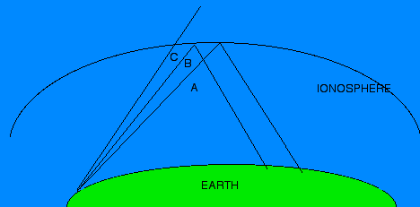
In the above picture, paths A and B are at shallow enough angles that the radio waves get reflected back to the Earth. For path C, the angle is too steep, and the radio waves are not reflected, but pass into space.

During the daytime, the ionosphere is able to support propagation of higher frequencies. As the sun sets and the ionization levels start to decrease, the maximum frequency begins to drop. For a given frequency, shorter transmission path distances will be affected first. The path will “close” very suddenly, sometimes over the span of just a few minutes or even seconds.

Here is a graph plotting the received signal level for WFMT on Dec 10, 2011:

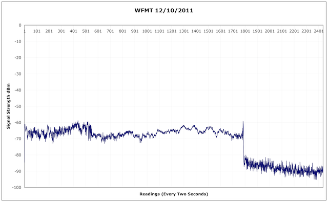
The signal strength is shown in dBm. Refer to the previous entry How many watts do you need? for a refresher course in dBm. In general, an S9 signal is -73 dBm, every S unit is theoretically 6 dB, so S8 is -81 dBm, etc.

You can see that the signal was varying between -60 and -70 dBm, so about S9+10 dB. Then quite suddenly, it dropped to about -85 dBm, and then continued to decline to about -90 dBm.

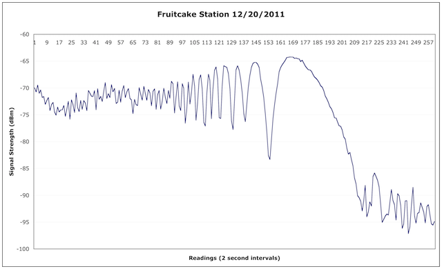
Here is a closeup graph showing one minute of signal strength during the time WFMT went long. You can see that it went long between 20 and 30 seconds. That is, it only took 10 seconds.

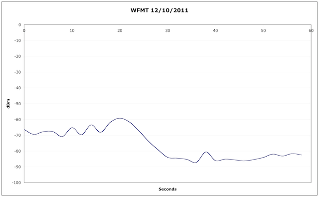
Looking carefully, you’ll also observe an increase in signal level just before WFMT went long. I have noticed this many times. My theory is that propagation is best when the incident angle of the radio waves to the ionosphere is very close to the critical angle. In this case, the incident angle is of course fixed, but the critical angle is changing as the ionosphere weakens to nighttime levels.

Note that even though the critical angle was exceeded, some radio waves are still being reflected, as the signal level has not dropped to zero yet (although it does continue to trend down, at some point the station will completely fade out).

The critical angle determines the maximum frequency that can be propagated between two points.

Remember from above that the maximum frequency that can be propagated is equal to foF2 divided by the sine of the angle. We can use some simple math to calculate what frequencies will work, knowing foF2.

The Maximum Usable Frequency (MUF) can be found by:
MUF = foF2 * sqrt( 1+ [D/(2*hmF2)]^2)

Where hmF2 is the height of the F2 layer. There is a map of the F2 height here:
http://www.spacew.com/www/hmf2.gif

For example, if the distance between the two stations is 690 km, and the F2 height is 250 km, and foF2 is 3.5 MHz, then plugging into the above formula gives us a MUF of 5.97 MHz. So we can use frequencies up to that. But, if the stations were closer together, say 300 km, then the MUF is only 4.1 MHz. (Note: It’s for long distances, it is important to remember that the signal probably takes several hops, and you need to use a value of D that is the distance between stations divided by the number of hops)

Note that like foF2, hmF2 is continuously varying. At 1600 UTC on December 14, 2011, the foF2 is about 9 MHz over the eastern USA, and the mmF2 is about 240 km. So 43 meters is potentially open to anywhere on the east coast, even using NVIS. Of course this only takes the MUF into account, there is also the LUF, or Lowest Usable Frequency, which is mostly a function of transmitter power and D layer absorption.

At night, foF2 dramatically drops. Lately it has been going below 7 MHz in around 2300 UTC, turning off NVIS for 43 meter band transmissions. With an foF2 of 6 MHz (observed today at 2330z) the MUF is around 7 MHz for a distance of 200 miles.

For this reason, operators who want to reach their target area (east coast ops reaching east coast listeners) should consider using lower frequencies at nighttime. Years ago, the 3 MHz band was somewhat popular for pirate operations. Even somewhere in 5 MHz would be useful.

NVIS itself is worthy of an entry by itself, which is coming up next.

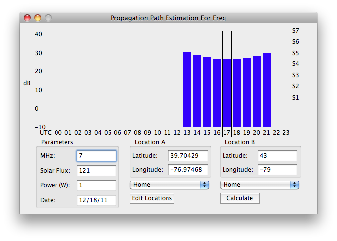
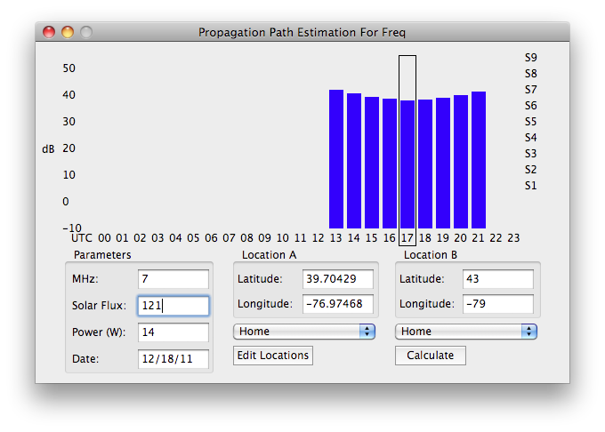
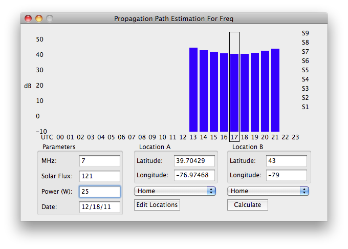
If you’re interested in getting real time propagation information, take a look at DX ToolBox which is available for both Windows and Mac OS X.