Graphs of Realtime HF Signal Levels

While it’s useful to forecast propagation conditions, it’s even more useful to know what the actual propagation conditions are. Propagation forecasting is somewhat like weather forecasting, although slightly less accurate.

I wanted to measure (and store for future reference) the signal levels from several shortwave stations from various parts of the world, transmitting on a range of frequencies. These stations can act as references for determining what propagation conditions are like to that part of the world, on a certain frequency or band, anyway.

One way to do this would be to step a radio through a list of frequencies, measuring the signal level and recording it. The problem is that you need to sit on a given frequency for at least some short period of time, to measure the signal level. And, if you’re only on the frequency for a second or two, that recorded signal level may not be characteristic of the actual signal level. You could have been monitoring while there was a burst of interference, causing a false high signal level reading. Or during a sudden deep fade, causing a weaker signal. And the longer you sit on one frequency, the less time you’re spending on other frequencies. You’re not continuously monitoring, but taking short snapshots.

But there is a solution. Once again, SDR (Software Defined Radio) to the rescue!

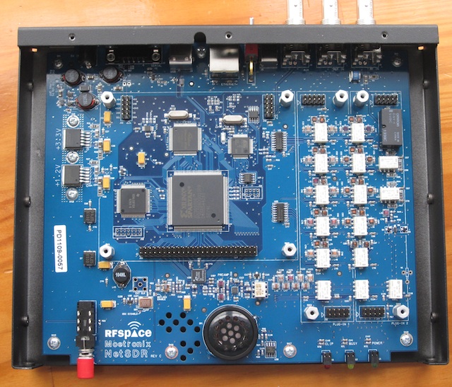
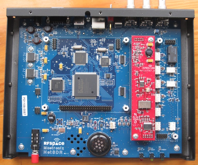
In this setup, an RF Space SDR-14 Software Defined Radio is connected to a 132 ft T2FD (Tilted Terminated Folded Dipole) antenna.

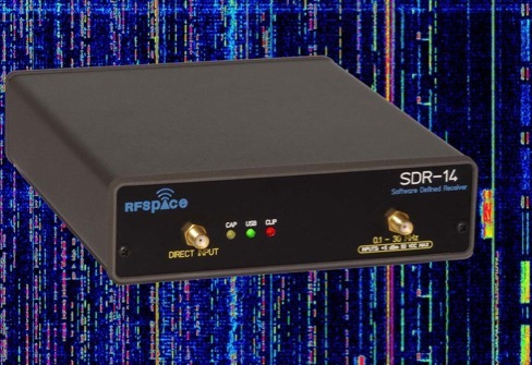
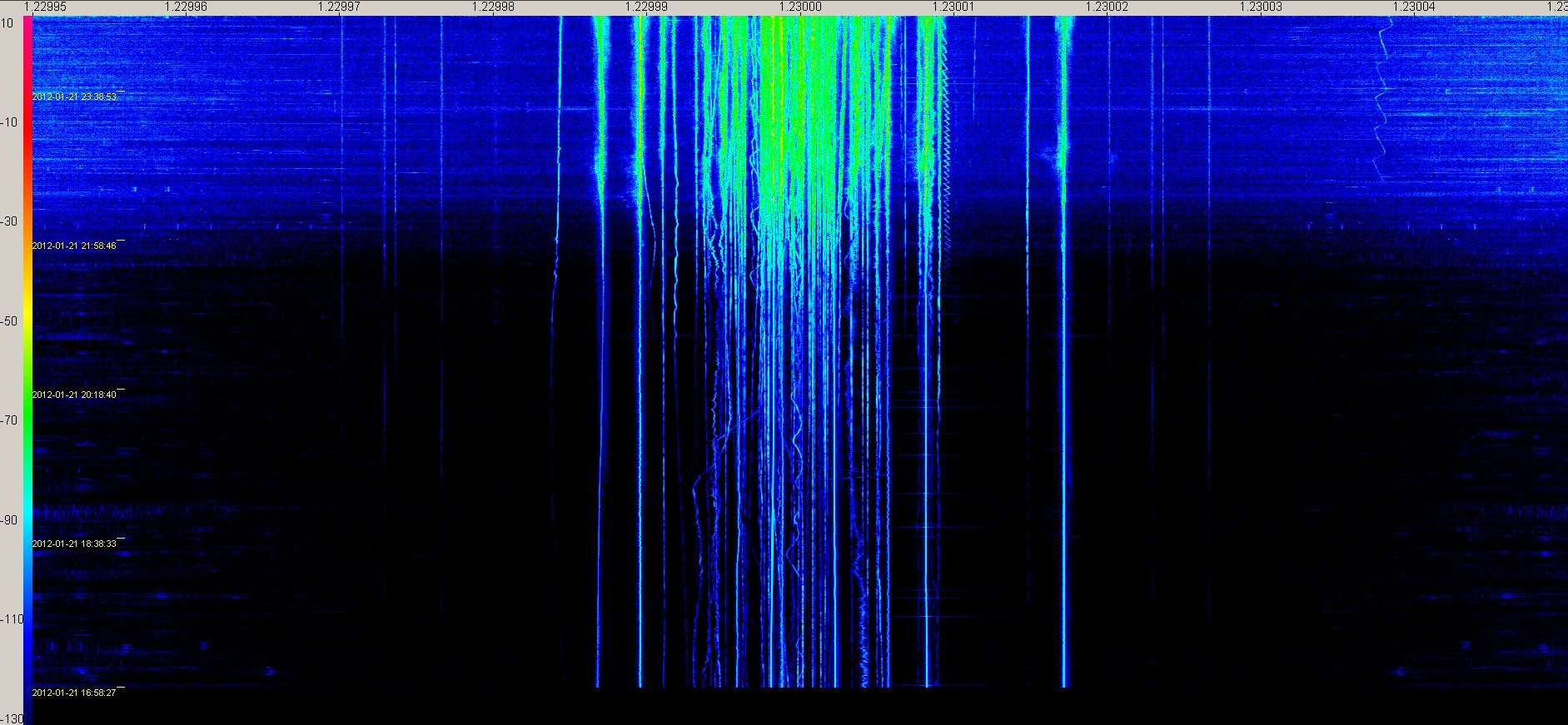
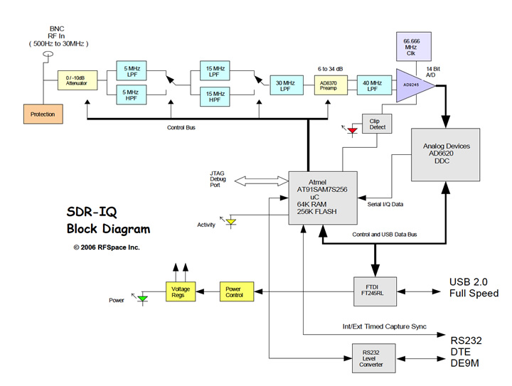
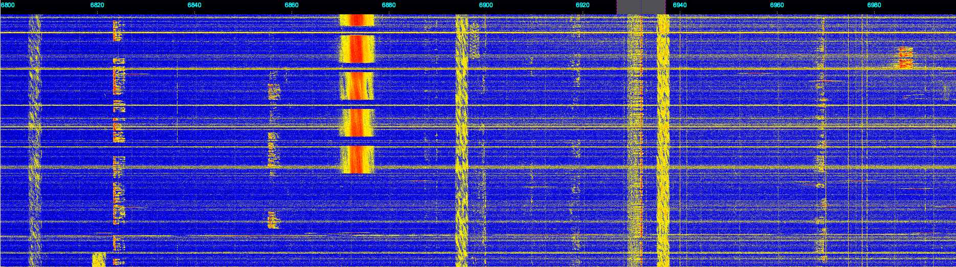
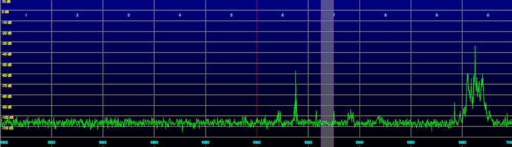
Custom software is continuously reading A/D (Analog to Digital Converter) values from the SDR-14 (in real, not complex, mode). The A/D sample rate is approximately 66.67 MHz. Blocks of 262,144 readings are taken, and an FFT is performed. The result is an array of signal strength readings for the entire HF spectrum, 0 to 30 MHz, in 254 Hz steps.

spectrum

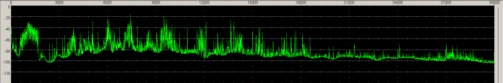
For frequencies of interest, the software then computes the signal strength in dBm over a +/-3 kHz bandwidth around a center frequency. This is computed approximately twice per second, and these readings are averaged over one minute. They are then uploaded to the web server, where they are stored, and graphs are made on demand when a user loads the page. These graphs show the last three days worth of readings. (Possibly less if I just started taking readings for that frequency)

The URL for accessing the graphs is http://www.hfunderground.com/propagation/

You will get a list of frequencies, with a brief description of the station on that frequency. Click on a frequency to get a graph of about three days worth of signal readings.

Several things can be readily observed:

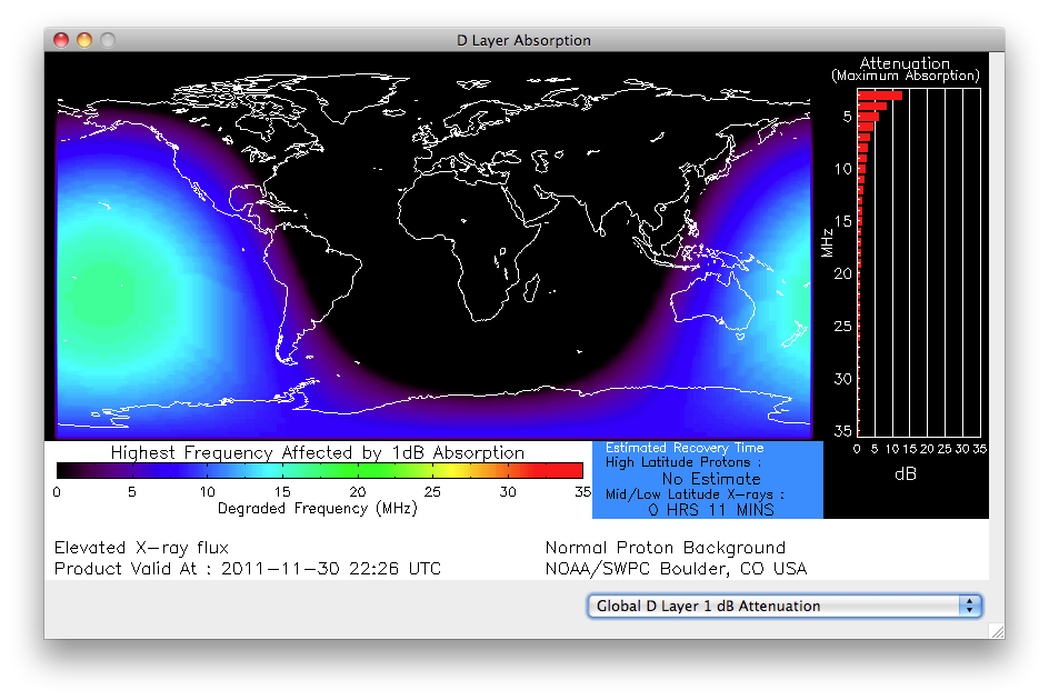
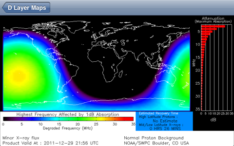
For the lower HF frequencies, signal levels are very weak during the daytime, due to absorption by the D layer. They then slowly rise as the Sun sets, stay high overnight, and then go back down again as the Sun rises.

For higher frequencies, say 6 and 7 MHz stations operating in NVIS mode such as NAA on 6726 kHz, you can see a sudden decrease in the signal level as the station goes long in the evening, and then an increase again when the Sun rises, and the F layer increases in strength. The signal does not always completely go away during the night, but it is significantly weaker. There are also periods at night when the signal level goes up and down. This could be the actual signal from the intended station, or possibly another station located elsewhere in the world.

The effect is much more pronounced for even higher frequencies, such as WWV on 20 MHz.

The recording for 10 MHz often shows WWV cutting out around local midnight, then the signal level goes back up again in the early morning, but before sunrise. I believe in this case we’re actually getting a signal from WWVH in Hawaii.

I’m also recording 25,555 kHz, which is a mostly open channel. My goal is to observe radio noise from Jupiter on this frequency.

The aviation weather frequencies (6604 kHz for example) do not have continuous transmissions, there are gaps. This is readily observable by seeing the steps in signal level.

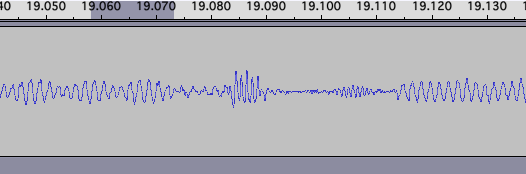
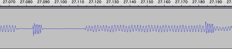
You will often see spikes in the graphs. This is mostly likely due to local noise, it could also be to brief transmissions on the frequency. There are ionospheric sounders that sweep across HF, as these pass by the frequencies being observed, they will cause a brief increase in the measured signal level.

You may also notice occasional gaps in data, the ancient computer the SDR-14 is running on (under Windows 2000) seems to develop USB issues every dozen or so hours. I need to try to set it up on another computer and see if that helps. Worst case I may try to rig up some sort of a Watchdog Timer.

Update: I’ve replaced the Win2k machine with a slightly less ancient machine running XP. We’ll see if that improves reliability. I know, reliability and Windows are rarely used in the same sentence. If only I knew someone with realtime OS experience like QNX…

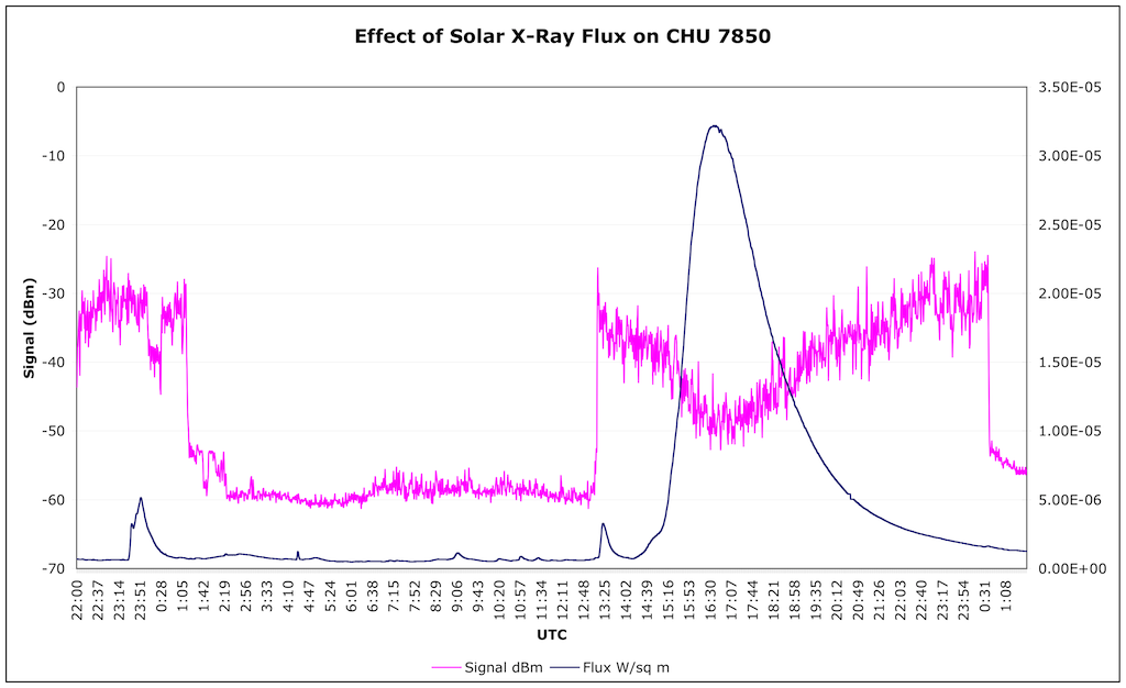
As mentioned during the introduction, these graphs can be very useful in determining what time of the day propagation is open to various parts of the world on certain bands. It is important to remember that much like the weather, propagation changes from day to day, and with the seasons. The levels of solar activity, as well as the effects of solar flares, have a dramatic effect on propagation. Changes in the season affect the number of hours per day of sunlight on the ionosphere over the different parts of the Earth, and cause seasonal changes to propagation patterns.

Do you have a suggestion for a frequency to monitor? Ideally, the frequency should have a station that is on 24 hours a day. If so, please pass it along!

An Afternoon in the 1230 kHz Graveyard

Below is a waterfall of 1230 kHz, captured with the netSDR. The recording starts just before 1700 UTC (at the bottom of the image) and runs until about 0030 UTC (top of the image), click on the image to expand it:

The total frequency width of the graph is 100 Hz, that is it extends +/-50 Hz from 1230 kHz. Now that I have the Rubidium Reference on the netSDR, I don’t have an issue with the radio itself drifting over time.

1230 kHz is a “graveyard” medium wave frequency in the US. There are six graveyard channels, 1230, 1240, 1340, 1400, 1450, and 1490 kHz. These channels were set aside as local channels by the North American Radio Broadcasting Agreement, which went into effect in 1941. The term graveyard comes from the weird mix of sounds often heard at night, as dozens of stations mix together. Graveyard stations are restricted to 1000 watts maximum, and some use well under that at night, sometimes under 100 watts.

As you can see by the graph, even at 1700 UTC (local noon) there are dozens of carriers present. Locally I have WRBS 33 miles away and WKBO 40 miles away. Within around 100 miles, there’s quite a few stations.

As it gets later and the D layer starts to go away, new stations appear, and the existing stations get stronger. At about 2200 UTC (5 PM local time) the background noise becomes more obvious as well.

Two of new carriers have an interesting sawtooth pattern to the carrier frequency.

The FCC requires a +/-20 Hz frequency accuracy for medium wave broadcast station carriers. It looks as though most if not all of the stations maintain that, it is impossible to say for sure what some of the outliers are, they could be MW stations or they could be a semi local QRM.

Adding a Rubidium Reference to the netSDR

I recently acquired a FE-5680 rubidium frequency reference off eBay. This is a high stability 10 MHz frequency reference. I also bought the REFCLOCK option for the netSDR directly from RF-Space, which takes the 10 MHz as a reference input, and produces an 80 MHz clock for the A/D, locked to the reference input. The result is less drift in the radio. The stock netSDR drift is already extremely low, but I want to do some observations of RF carriers over a long time period, so I wanted to reduce the drift even further.

Here’s a picture of the reference I bought, it was around $55 shipped, from China of course.

The reference requires 16V at just under 2A peak, as well as 5V at a lower current. I used an old laptop power supply, and rigged a 7805 to produce the 5V. Unfortunately all input and output is via a DB-9 connector. The 16V is applied via the barrel connector on the left, and the 10 MHz comes out the BNC on the right.

Here’s the inside of the netSDR receiver:

And after installing the REFCLOCK module:

I’ll post some followup articles with long term waterfalls, and we’ll see how the drift looks.

But how does the rubidium frequency reference work? From the FE-5680 technical manual:

The Rubidium Physics Package incorporates a rubidium cell, rubidium lamp, and servo electronics to utilize the ground-state hyperfine transition of the rubidium atom, at approximately 6.834x GHz.The VCXO is locked to the rubidium atomic resonance in the following manner. The VCXO frequency of 50.255x MHz is an exact sub-multiple (36) of the atomic resonance frequency at 6.834x GHz. A microwave signal, having a frequency in the vicinity of 6.834x GHz, is generated from the nominal 50.255x MHz VCXO input. This microwave signal is used to resonate vaporized rubidium atoms within a sealed glass Rb resonance cell that is placed in a low Q microwave cavity.

The microwave frequency generation method is designed so that the VCXO frequency is exactly 50.255x MHz when the microwave frequency is exactly equal to 6.834x GHz. The frequency of the signal applied to the microwave cavity can be maintained equal to 6.834x GHz by generating an error signal when the frequency varies, and using this error signal to servo the VCXO via its control voltage.

The error signal is generated in the physics package. Light from the rubidium lamp, produced by an excited plasma discharge, is filtered and passed through the rubidium resonance cell where it interacts with rubidium atoms in the vapor. After passing through the resonance cell, this light is incident upon a photocell. When the applied microwave frequency is equal to 6.834x GHz, the rubidium atoms are resonated by the microwave field in the cavity; this causes the light reaching the photocell to decrease. The decrease in light, when the microwave frequency is equal to the sharply defined Rubidium frequency, is then converted electronically to an error signal with phase and amplitude information that is used to steer the VCXO via its control voltage and keep it on frequency at 50.255x MHz.

The VCXO operates nominally at 50.255x MHz. The VCXO has two isolated outputs; one output is provided to the Rubidium Physics Package for comparison purposes, and the other output is used as the clock input for direct digital synthesis within the Synthesizer.

The Effects of a Solar Flare on CHU Reception

Here’s a graph of the signal strength of CHU 7850 kHz (the Canadian time station) recorded from 2200 UTC on January 18, 2012 to 0100 UTC on January 20, 2012, the signal strength is the pink line, and is in dBm. Also shown on the graph is the solar x-ray flux level, as measured by the GOES 15 weather satellite (click on the graph for a larger image):
CHU 7850 Signal Graph

The recording was made with an SDR-14 set to record a 5 kHz bandwidth (8137 Hz sampling rate) centered on 7850 kHz. This was AM demodulated with the IF filter set to cover 7849.7 to 7852.5 kHz, covering the carrier as well as much of the modulated signal. CHU transmits a carrier and upper side band, with 10 kW of power. The displayed dBm readings are too high by 24 dB, due to the IF gain setting on the SDR-14. I’ll need to correct for that with future recordings. But the relative changes are valid.

We can observe a few things here. First, there are three sudden changes in signal strength:

At 0114 UTC, the signal suddenly dropped by about 25 dB, this is when the band went long. It then further dropped another 6 dB or so.

At 1312 UTC, the signal suddenly came back up, this is when F layer ionization was strong enough again for reception of CHU via NVIS.

At 0038 UTC, the signal dropped again when the band went long. Note that this occurred at a different time than the night before.

For reference, CHU is about 550 km from my location.

The big event on the 19th was the solar flare. It peaked at a level of M3.2, and was a very long duration flare, it stayed at M levels from about 1500 to 1930 UTC. You can see the effects on CHU, the signal dropped about 2 S units (12 dB). The effects on CHU’s 90 meter frequency of 3330 kHz were even more dramatic, I tried tuning in, and it was completely gone. Normally it is S9 or better during the daytime in the winter.

The attenuation was due to the x-rays from the flare increasing the ionization of the D layer of the ionosphere. The D layer does not contribute to propagation, rather it attenuates radio waves. So a stronger D layer means weaker signals, and the effect is more pronounced at lower frequencies.

You’ll notice a dip in the signal around 2300 UTC on the first day, and a small solar flare about the same time. I believe this is a coincidence, not due to the flare. The decrease in signal is too sudden, and the flare was not that large. I quickly put up a special dipole for this test, and it may have some issues. We had some wind that day, perhaps there was an intermittent contact.

While we didn’t have any flares overnight, if we had, there would not have been an affect on the signal, as they only affect the part of the Earth in sunlight, and this path was entirely in the dark side of the Earth.

What’s All This SDR Stuff, Anyhow?

The Software Defined Radio (SDR) has become very popular in the radio hobby scene over the last few years. Many hobbyists own one, certainly most have heard of them. But what is an SDR, and why might you want one, over a traditional radio?

First, a very brief explanation of how the traditional superhetrodyne radio works. This is the type of radio you have, if you don’t have an SDR (and you don’t have a crystal radio).

Here’s a block diagram of a typical superhetrodyne receiver:

superhetrodyne block diagram

The antenna is connected to a RF amplifier, which amplifies the very weak signals picked up by the antenna. Some high end radios put bandpass filters between the antenna and RF amplifier, to block strong out of band signals which could cause mixing products and images.

Next, the signals are passed to a mixer, which also gets fed a single frequency from the local oscillator. A mixer is a non linear device that causes sum and difference frequencies to be produced. I won’t go into the theory of exactly how it works. The local oscillator frequency is controlled by the tuning knob on the radio. It is offset by a fixed amount from the displayed frequency. That amount is called the IF frequency. For example, the IF of an radio may be 455 kHz. Time for an example…

Say you’re tuned to 6925 kHz. The local oscillator generates a frequency of 6470 kHz, which is 455 kHz below 6925 kHz. The mixer mixes the 6470 kHz signal with the incoming RF from the antenna. So the RF from a station transmitting on 6925 kHz gets mixed with 6470 kHz, producing a sum (6925+6470=13395 kHz) and difference (6925-6470=455 kHz) signal. The IF Filter after the mixer only passes frequencies around 455 kHz, it blocks others. So only the difference frequencies of interest, from the 6925 kHz station, get paseed. This signal is then amplified again, fed to a demodulator to convert the RF into audio frequencies, and fed to an audio amplifier, and then the speaker. The IF filter is what sets the selectivity of the radio, the bandwidth. Some radios have multiple IF filters that can be switched in, say for wide audio (maybe 6 Khz), and narrow (maybe 2.7 kHz). Perhaps even a very narrow (500 Hz) filter for CW.

This is a very basic example. Most higher end HF radios actually have several IF stages, with two or three being most common. The Icom R-71A, a fairly high end radio for its time (the 1980s) had four IF stages. Additional IF stages allow for better filtering of the signal, since it is not possible to build real physical filters with arbitrary capabilities. There’s a limit to how much filtering you can do at each stage.

Now, onto the SDR. I’ll be describing a Direct Digital Sampling (DDS) style SDR. The other style is the Quadrature Sampling Detector (QSD), such as the “SoftRock” SDR. The QSD SDR typically mixes the incoming RF to baseband, where it is then fed to the computer via a sound card interface for processing. The main advantage of the QSD SDR is price, it is a lot cheaper due to fewer components. The sacrifice is performance and features. You can’t get more than about 192 kHz bandwidth with a sound card, and you suffer from signal degradation caused by the sound card hardware. Some try to compensate for this by buying high end sound card interfaces, but at that point you’re approaching the price point of a DDS SDR in total hardware cost anyway.

Here is a block diagram of the SDR-IQ, courtesy of RF Space, you can click on it to see an enlarged image.
sdr-iq block diagram

The RF input (from the antenna) goes in at the left end, much of the front end is the same as a traditional radio. There’s an attenuator, protection against transients/static, and switchable bandpass filters and an amplifier. Finally the RF is fed into an A/D converter clocked at 66.666 MHz. An A/D (Analog to Digital) Converter is a device that continuously measures a voltage, and sends those readings to software for processing. Think of it as a voltmeter. The RF signals are lots of sine waves, all jumbled together. At a very fast rate, over 66 million times per second in this case, the A/D converter is measuring the voltage on the antenna. You’ve got similar A/D converters on the sound card input to your computer. The difference is that a sound card samples at a much lower rate, typically 44.1 kHz. So the A/D in an SDR is sampling about a thousand times faster. It is not too much of a stretch to say that the front end of an SDR is very similar to sticking an antenna into your sound card input. In fact, for many years now, longwave radio enthusiasts have used sound cards, especially those that can sample at higher rates such as 192 kHz, as SDRs, for monitoring VLF signals.

The output of the A/D converter, which at this point is not RF but rather a sequence of voltage readings, is fed to the AD6620, which is where the actual DSP (Digital Signal Processing) is done. The AD6620 is a dedicated chip for this purpose. Other SDRs, such as the netSDR, use a device called a FPGA (Field Programmable Gate Array), which, as the name implies, can be programmed for different uses. It has a huge number of digital logic gates, flip flops, and other devices, which can be interconnected as required. You just need to download new programming instructions. The AD6620 or FPGA does the part of the “software” part of the SDR, the other part being done in your computer.

The DSP portion of the SDR (which is software) does the mixing, filtering, and demodulation that is done in analog hardware in a traditional radio. If you looked at a block diagram of the DSP functions, they would be basically the same as in a traditional radio. The big advantage is that you can change the various parameters on the fly, such as IF filter width and shape, AGC constants, etc. Automatic notch filters become possible, identifying and rejecting interference. You can also realize tight filters that are essentially impossible with actual hardware. With analog circuitry, you introduce noise, distortion, and signal loss with each successive stage. With DSP, once you’ve digitized your input signal, you can perform as many operations as you wish, and they are all “perfect”. You’re only limited by the processing power of your DSP hardware.

Since it is not possible feed a 66 MHz sampled signal into a computer (and the computer may not have the processing power to handle it), the SDR software filters out a portion of the 0-30 MHz that is picked up by the A/D by mixing and filtering, and sends a reduced bandwidth signal to the computer. Often this is in the 50 to 200 kHz range, although more recent SDRs allow wider bandwidths. The netSDR, for example, supports a 1.6 MHz bandwidth.

With a 200 kHz bandwidth, the SDR could send sampled RF to the computer representing 6800 to 7000 kHz. Then additional DSP software in the computer can further process this information, filtering out and demodulating one particular radio station. Some software allows multiple stations to be demodulated at the same time. For example, the Spectravue software by RF Space allows two frequencies to be demodulated at the same time, one fed to the left channel of the sound card, and one to the right. So you could listen to 6925 and 6955 kHz at the same time.

Another obvious benefit of an SDR is that you can view a real time waterfall display of an entire band. Below is a waterfall of 43 meters at 2200 UTC (click on it to enlarge):
43 meter band waterfall

You can see all of the stations operating at one glance. If a station goes on the air, you can spot it within seconds.

Finally, an SDR allows you to record the sampled RF to disk files. You can then play it back. Rather than just recording a single frequency, as you can with a traditional radio, you can record an entire band. You can then go back and demodulate any signals you wish to. I’ll often record 6800 to 7000 kHz overnight, then go back to look for any broadcasts of interest.

For brevity, I avoided going into the details of exactly how the DSP software works, that may be the topic of a future post.

And yes, I borrowed the “What’s All this… Stuff, Anyhow” title from the late great Bob Pease, an engineer at National Semiconductor, who wrote a fabulous series of columns under that title at EDN magazine for many years.

Propagation Tools – Monitoring Background X-Ray Flux Levels

The GOES 15 weather satellite (the one that is in geostationary orbit and provides the animated views of the weather over the US that you often see on the TV news) also has a set of sensors that monitor the Sun. One of these measures the x-ray output.

These x-rays are produced by sunspots, as well as by solar flares. The x-ray flux we’re interested in is measured in the 1 to 8 Angstrom range (that is the wavelength) and is the red line on the graph below (the blue line is the 0.5 to 4 Angstrom range, x-rays of a shorter wavelength):
x-ray flux

The URL for this graph is http://www.swpc.noaa.gov/rt_plots/Xray.gif

In addition, there is a graph that updates at a 1 minute rate, located at http://www.swpc.noaa.gov/rt_plots/Xray_1m.gif

x-ray flux 1 minute

X-ray level measurements consist of a letter and number, such as B6.7, representing the x-ray flux in watts/square meter. It is a log scale, much like what is used for earthquakes. A value of C1.0 is ten times as large as B1.0 (and would be equivalent to B10). Values in the A range are low background levels, such as at solar minimum. B values are a moderate background, and C values are either a high background or solar flare conditions. Flares usually result in short bursts of large x-ray levels, in the C, M, or even X range. Remember that this is a log scale, so an M1 flare is 10 times as energetic as a C1 flare, and an X1 flare is 100 times. There is a new Y classification as well, so a flare that would have been say X28 in the past would now be Y2.8.

These x-rays ionize the D layer of the ionosphere, which attenuates radio waves. So high x-ray flux levels increase attenuation of radio waves, especially at lower frequencies. Below is a map of D layer absorption:
http://www.swpc.noaa.gov/drap/Global.png

The x-rays also increase the ionization of the F layer (which is the layer that gives us shortwave propagation), although the effect is less than for the D layer.

The net result is that increased x-ray levels cause more attenuation at lower frequencies, but can also lead to better propagation at higher frequencies. Long periods of high x-ray flux levels (well into the C range) may be a sign of good 10 and 6 meter band conditions. I’ve also found that high (C range) levels seem to “stir the pot” for MW DX, bringing in different stations than usual.

Very high flux levels, such as during a major flare (in the high M or X range) however cause radio blackouts. These occur first as lower frequencies, and as the D layer begins to get more ionized higher frequencies are also affected. Extremely energetic flares (X range) can wipe out all of HF. Note that this is only true for propagation paths on the sunlight side of the Earth. The dark side is not affected. This means that flares can be useful at times, in that they can cause the fadeout of an interfering dominant station on a particular frequency, allowing another station to be heard, providing the geometry of the Earth and Sun are correct such that the path of the interfering station is in the sunlit part of the Earth, while the other station is not.

Solar flares are usually of a short duration, minutes to an hour, although there are “long duration events” that can last for several hours. If you notice suddenly poor conditions, you may want to check the current x-ray flux levels, to see if a flare is the cause. If so, try higher frequencies, as they are less affected.

As we are finally nearing the maximum of Solar Cycle 24 (although it appears it will be a fairly weak maximum) we can expect to see more flares. It can be very handy to continuously monitor the x-ray flux and D layer absorption levels, to see what the current conditions are, and to take advantage of them. One handy way to do this is with DX Toolbox. With DX Toolbox, you can monitor the current conditions, and even get an alert when the x-ray flux exceeds a predetermined alarm value. Some screenshots are below, click on them for a larger image:

DX Toolbox is available for Windows and the Macintosh, you can download a copy at this URL: http://www.blackcatsystems.com/download/dxtoolbox.html

There is also an iOS version available for the iPhone, iPad, and iPod:

Visit this URL for more information:http://www.blackcatsystems.com/iphone/dx_toolbox.html or go directly to the iTunes Store

DX Toolbox also has several propagation prediction windows, to help estimate signal levels for any path you enter, based on solar conditions.

A Day In The Life of 1470 kHz

This waterfall was recorded from 1840 UTC January 3, 2011 to 1840 UTC January 4, 2011. The beginning of the recording is at the top of the image. It shows the carriers of MW radio stations on 1470 kHz. The width is 100 Hz, so frequencies +/-50 Hz from 1470 kHz are shown.

Click on it to open it full sized.

1470 kHz Waterfall

The red line you see in the center is the carrier of semi-local station WTTR. During the daytime it is the only audible station on 1470, although you can see that carriers for about 8 other stations are always present.

I’ve annotated several events with UTC times.

At about 2213 UTC you can see a sudden reduction in received signal strength, and the start of a drift in frequency. This is most likely due to a station switching to nighttime power levels. The change in transmitter power causes a change in temperature inside the transmitter, causing drift in the frequency. My suspicion is that it is WLOA from Farrel, PA, since they are supposed to switch at 2215 UTC.

At about 2252 UTC a carrier suddenly disappears. It is possible that this is KMAL from Malden, MO. They are supposed to shut down at 2300 UTC.

Note that these are hunches of mine, I am not 100% certain that these are the identified stations. These events do suggest that it may be possible to identify and DX stations based on carrier transients, if the actual times that the stations make the changes are known.

At 0400 UTC a carrier suddenly disappears. I am not sure who this could be. This would be 11 PM EST. The station started to fade in around 2300 UTC (6 PM EST). That suggests to me a station in the central US. I’m not sure why they would be shutting down at this late time of the evening, vs around sunset. Perhaps some more experienced MW DXers have some theories / candidates?

There’s also some transients in the morning.

First at around 1200 UTC (7 AM local time) you can see the received signal strengths of the distant carriers decrease. The Sun is rising, and the D Layer is forming again, attenuating MW skywave signals.

At 1230 UTC one of the carriers suddenly disappears. At 1251 a carrier appears.

At 1326, it looks like a a transmitter is changing power levels.

At 1406 UTC there is another transient on another carrier.

There’s also noticeable differences in the frequency regulation of transmitter carriers. Several of the carriers have a periodic cycling to the frequency. I thought is this is due to some temperature cycling in the transmitter.

The 1610 Zoo

Below is a waterfall centered around 1610 kHz in the extended MW (AM) Band, 100 Hz Wide (click on it to see an enlarged image): 1610 waterfall

1610 kHz is used by only two broadcast stations, both in Canada: CJWI in Montreal, and CHHA in Toronto. It is also, however, used by many TIS (Travelers Information Stations) stations, which broadcast traffic reports, weather, etc. These are low power stations, typically in the 10 watt range.

Locally, the dominant station on 1610 kHz is a TIS that relays NOAA weather transmissions, and is located somewhere in south central PA. I’ve never heard an ID.

This recording was made between about 2100 and 1700 UTC, you can see the increase in signal (and background) levels overnight, and then the weakening of the signals as the Sun rises and the D Layer reforms, attenuating distant stations. Looking at the waterfall, you can see dozens of carriers, each a different radio station. It’s interesting to note how many radio station signals are present, even during the daytime.

The horizontal lines are due to static bursts, and there’s some changes in the signal level due to the wind blowing around the antenna.

Some of the wandering of carriers you see that is in unison is due to drift of the A/D clock in the SDR. Other drift you see is due to the carriers themselves. Note that each major division at the top of the waterfall is only 10 Hz (and the entire width is 100 Hz) so there’s really only a few Hz total drift. Eventually I’ll get a more stable reference clock for the SDR, and receiver drift should go away.

Let’s have a contest. How many carriers can you count?

Measuring The Speed of Light Using a Shortwave Radio

I thought it would be interesting to see whether or not it was possible to crudely measure the speed of light using a shortwave radio and a time station.

Various time stations transmit precise time on several shortwave frequencies. Here in the USA, we have WWV in Ft. Collins, Colorado, which transmits on 2.5, 5, 10, 15, and 20 MHz. We also have WWVH in Kekaha, Hawaii, which transmits on 2.5, 5, 10, and 15 MHz. These stations transmit an audio “tick” at exactly each UTC second.

One way to measure the speed of radio waves (and light) would be to measure how long it takes for the tick to travel a fixed distance. Divide the distance by the time, and we have the speed of light. However, that requires knowing the exact UTC time locally. While this can be done with a GPS unit that outputs a 1 PPS (pulse per second) signal, I thought it would be more interesting to do it using just a shortwave radio without any extra hardware, other than a computer to record the audio.

Both WWV and WWVH transmit on several of the international time frequencies. And it turns out that at certain times of the day, it is possible to receive both of them on the same frequency. The following recording was made on 15 MHz at 1821 UTC on January 1, 2011: Recording of WWV and WWVH

You can hear the time announcement for WWVH first, by a woman, followed by a man giving the WWV time announcement.

I am roughly at a location of 77W and 40N. WWV is located at roughly 105W and 41N, and is about 2,372 km away. WWVH is located at roughly 160W and 22N, about 7,883 km away. The actual path the radio waves takes to reach me is longer, due to the fact that they reflect off the ionosphere, a few hundred km high. We’ll neglect that for now.

The difference in distance between WWV and WWVH is 7883 – 2372 = 5510 km.

The following is a display of the waveform from the above recording, centered around one of the second ticks. You can see the stronger WWV second tick centered at about 19.086 seconds into the recording. You can also see the weaker WWVH second tick centered at about 19.105 seconds: wwv and wwvh

The other waveforms you see before and after the second ticks are the audio that each station always transmits.

If we subtract the time markers for the two ticks, we get 19.105 – 19.086 = 0.019 seconds (19 milliseconds). That’s the time delay between the two ticks. Next, performing our division, 5510 km / 0.019 seconds = 290,000 km/second. The generally accepted value for the speed of light is 299,792 km/second. That’s pretty close!

In all fairness, the time resolution is not that good, and I had to eyeball the readings. Plus, a one millisecond difference in the time delay would have resulted in about a 15,000 km/sec difference in the speed of light. So a slight difference in eyeballing these broad time ticks would result in a large error in our estimate of the speed of light.

If you listened carefully to the recording, you no doubt heard a fluttery or watery quality to the sound. This is often indicative of multipath, where the radio waves take two (or more) paths between the transmitter and receiver.

Here’s another waveform from the recording, centered at 27 seconds into the recording: wwv and wwvh long path

In this case, we can clearly see the second tick from WWVH. But there’s no second tick from WWVH, just silence. Where is it?

Looking further into the recording, we see another second tick delayed much further. Eyeballing it, the delayed tick is at about 27.187 seconds into the recording. And the first tick, which we believe is from WWV is at about 27.087 seconds. The difference between the two is 0.100 seconds. Using the accepted speed of light, this difference in time could be due to a distance of 299,792 km/sec * 0.100 sec = 29,972 km. What could account for this delay?

One possibility is that during this time period, the signal from WWVH was not taking the normal or short path to my location, but was instead travelling around the other side of the Earth, taking the long path.

The circumference of the Earth is about 40,075 km (the exact value depends on which path around the Earth you take, as the Earth is not a perfect sphere). We know the short path is 7,883 km, so the long path is about 40075 – 7883 = 32192 km. There is still the delay due to the time it takes the radio waves to get from WWV to my location, that path is 2,372 km. The net difference between the two is 32192 – 2372= 29820 km.

We can divide that distance by the speed of light to see what the time delay should be: 29820 km / 299792 km/sec = 0.099 seconds. This is extremely close to our measured period of 0.100 seconds, and suggests that the long delayed second tick really is from the WWVH signal taking the long path around the Earth to reach us.

The following map, generated with the DX ToolBox Radio Propagation Forecasting Program, shows both the short path (white line) and long path (gray line) between my location and WWVH: WWVH Path

Comments appreciated!