Propagation Tools – Monitoring Background X-Ray Flux Levels

The GOES 15 weather satellite (the one that is in geostationary orbit and provides the animated views of the weather over the US that you often see on the TV news) also has a set of sensors that monitor the Sun. One of these measures the x-ray output.

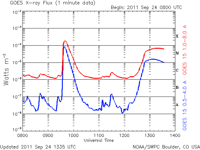
These x-rays are produced by sunspots, as well as by solar flares. The x-ray flux we’re interested in is measured in the 1 to 8 Angstrom range (that is the wavelength) and is the red line on the graph below (the blue line is the 0.5 to 4 Angstrom range, x-rays of a shorter wavelength):
x-ray flux

The URL for this graph is http://www.swpc.noaa.gov/rt_plots/Xray.gif

In addition, there is a graph that updates at a 1 minute rate, located at http://www.swpc.noaa.gov/rt_plots/Xray_1m.gif

x-ray flux 1 minute

X-ray level measurements consist of a letter and number, such as B6.7, representing the x-ray flux in watts/square meter. It is a log scale, much like what is used for earthquakes. A value of C1.0 is ten times as large as B1.0 (and would be equivalent to B10). Values in the A range are low background levels, such as at solar minimum. B values are a moderate background, and C values are either a high background or solar flare conditions. Flares usually result in short bursts of large x-ray levels, in the C, M, or even X range. Remember that this is a log scale, so an M1 flare is 10 times as energetic as a C1 flare, and an X1 flare is 100 times. There is a new Y classification as well, so a flare that would have been say X28 in the past would now be Y2.8.

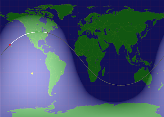
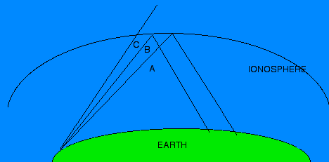
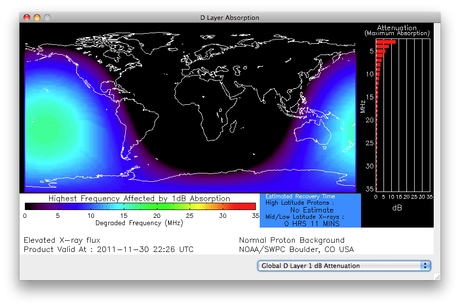
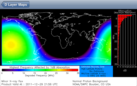
These x-rays ionize the D layer of the ionosphere, which attenuates radio waves. So high x-ray flux levels increase attenuation of radio waves, especially at lower frequencies. Below is a map of D layer absorption:
http://www.swpc.noaa.gov/drap/Global.png

The x-rays also increase the ionization of the F layer (which is the layer that gives us shortwave propagation), although the effect is less than for the D layer.

The net result is that increased x-ray levels cause more attenuation at lower frequencies, but can also lead to better propagation at higher frequencies. Long periods of high x-ray flux levels (well into the C range) may be a sign of good 10 and 6 meter band conditions. I’ve also found that high (C range) levels seem to “stir the pot” for MW DX, bringing in different stations than usual.

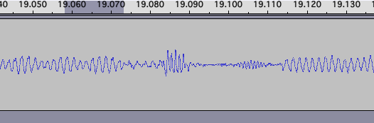
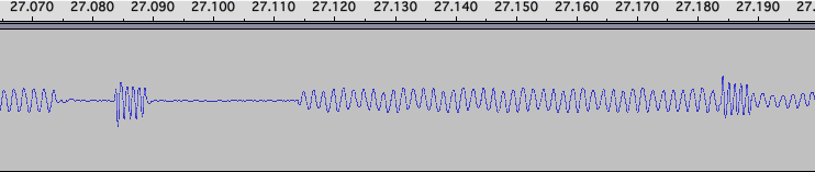
Very high flux levels, such as during a major flare (in the high M or X range) however cause radio blackouts. These occur first as lower frequencies, and as the D layer begins to get more ionized higher frequencies are also affected. Extremely energetic flares (X range) can wipe out all of HF. Note that this is only true for propagation paths on the sunlight side of the Earth. The dark side is not affected. This means that flares can be useful at times, in that they can cause the fadeout of an interfering dominant station on a particular frequency, allowing another station to be heard, providing the geometry of the Earth and Sun are correct such that the path of the interfering station is in the sunlit part of the Earth, while the other station is not.

Solar flares are usually of a short duration, minutes to an hour, although there are “long duration events” that can last for several hours. If you notice suddenly poor conditions, you may want to check the current x-ray flux levels, to see if a flare is the cause. If so, try higher frequencies, as they are less affected.

As we are finally nearing the maximum of Solar Cycle 24 (although it appears it will be a fairly weak maximum) we can expect to see more flares. It can be very handy to continuously monitor the x-ray flux and D layer absorption levels, to see what the current conditions are, and to take advantage of them. One handy way to do this is with DX Toolbox. With DX Toolbox, you can monitor the current conditions, and even get an alert when the x-ray flux exceeds a predetermined alarm value. Some screenshots are below, click on them for a larger image:

DX Toolbox is available for Windows and the Macintosh, you can download a copy at this URL: http://www.blackcatsystems.com/download/dxtoolbox.html

There is also an iOS version available for the iPhone, iPad, and iPod:

Visit this URL for more information:http://www.blackcatsystems.com/iphone/dx_toolbox.html or go directly to the iTunes Store

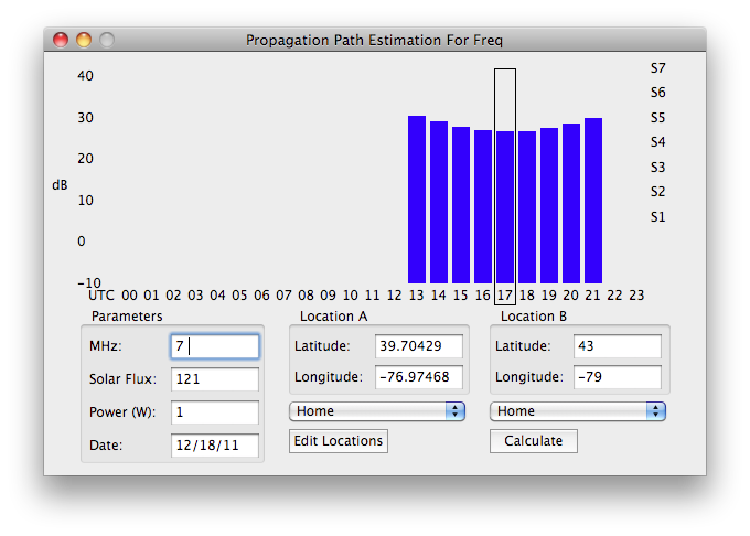
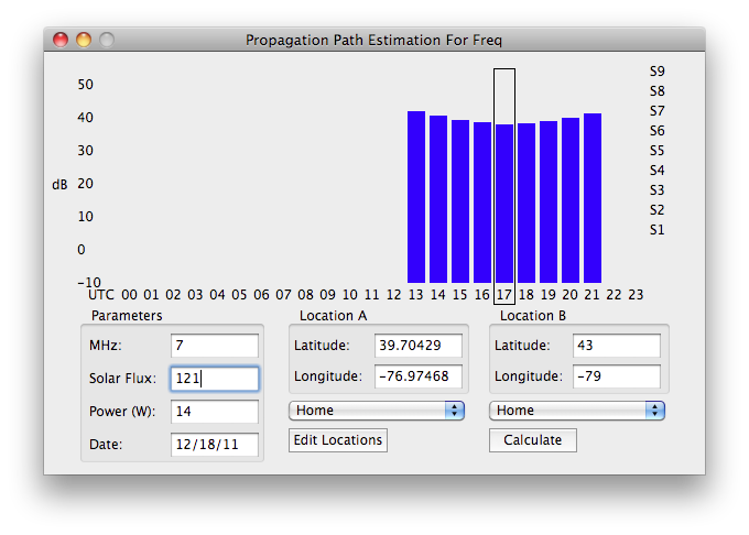
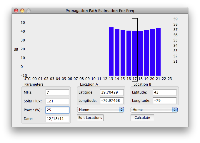
DX Toolbox also has several propagation prediction windows, to help estimate signal levels for any path you enter, based on solar conditions.

Measuring The Speed of Light Using a Shortwave Radio

I thought it would be interesting to see whether or not it was possible to crudely measure the speed of light using a shortwave radio and a time station.

Various time stations transmit precise time on several shortwave frequencies. Here in the USA, we have WWV in Ft. Collins, Colorado, which transmits on 2.5, 5, 10, 15, and 20 MHz. We also have WWVH in Kekaha, Hawaii, which transmits on 2.5, 5, 10, and 15 MHz. These stations transmit an audio “tick” at exactly each UTC second.

One way to measure the speed of radio waves (and light) would be to measure how long it takes for the tick to travel a fixed distance. Divide the distance by the time, and we have the speed of light. However, that requires knowing the exact UTC time locally. While this can be done with a GPS unit that outputs a 1 PPS (pulse per second) signal, I thought it would be more interesting to do it using just a shortwave radio without any extra hardware, other than a computer to record the audio.

Both WWV and WWVH transmit on several of the international time frequencies. And it turns out that at certain times of the day, it is possible to receive both of them on the same frequency. The following recording was made on 15 MHz at 1821 UTC on January 1, 2011: Recording of WWV and WWVH

You can hear the time announcement for WWVH first, by a woman, followed by a man giving the WWV time announcement.

I am roughly at a location of 77W and 40N. WWV is located at roughly 105W and 41N, and is about 2,372 km away. WWVH is located at roughly 160W and 22N, about 7,883 km away. The actual path the radio waves takes to reach me is longer, due to the fact that they reflect off the ionosphere, a few hundred km high. We’ll neglect that for now.

The difference in distance between WWV and WWVH is 7883 – 2372 = 5510 km.

The following is a display of the waveform from the above recording, centered around one of the second ticks. You can see the stronger WWV second tick centered at about 19.086 seconds into the recording. You can also see the weaker WWVH second tick centered at about 19.105 seconds: wwv and wwvh

The other waveforms you see before and after the second ticks are the audio that each station always transmits.

If we subtract the time markers for the two ticks, we get 19.105 – 19.086 = 0.019 seconds (19 milliseconds). That’s the time delay between the two ticks. Next, performing our division, 5510 km / 0.019 seconds = 290,000 km/second. The generally accepted value for the speed of light is 299,792 km/second. That’s pretty close!

In all fairness, the time resolution is not that good, and I had to eyeball the readings. Plus, a one millisecond difference in the time delay would have resulted in about a 15,000 km/sec difference in the speed of light. So a slight difference in eyeballing these broad time ticks would result in a large error in our estimate of the speed of light.

If you listened carefully to the recording, you no doubt heard a fluttery or watery quality to the sound. This is often indicative of multipath, where the radio waves take two (or more) paths between the transmitter and receiver.

Here’s another waveform from the recording, centered at 27 seconds into the recording: wwv and wwvh long path

In this case, we can clearly see the second tick from WWVH. But there’s no second tick from WWVH, just silence. Where is it?

Looking further into the recording, we see another second tick delayed much further. Eyeballing it, the delayed tick is at about 27.187 seconds into the recording. And the first tick, which we believe is from WWV is at about 27.087 seconds. The difference between the two is 0.100 seconds. Using the accepted speed of light, this difference in time could be due to a distance of 299,792 km/sec * 0.100 sec = 29,972 km. What could account for this delay?

One possibility is that during this time period, the signal from WWVH was not taking the normal or short path to my location, but was instead travelling around the other side of the Earth, taking the long path.

The circumference of the Earth is about 40,075 km (the exact value depends on which path around the Earth you take, as the Earth is not a perfect sphere). We know the short path is 7,883 km, so the long path is about 40075 – 7883 = 32192 km. There is still the delay due to the time it takes the radio waves to get from WWV to my location, that path is 2,372 km. The net difference between the two is 32192 – 2372= 29820 km.

We can divide that distance by the speed of light to see what the time delay should be: 29820 km / 299792 km/sec = 0.099 seconds. This is extremely close to our measured period of 0.100 seconds, and suggests that the long delayed second tick really is from the WWVH signal taking the long path around the Earth to reach us.

The following map, generated with the DX ToolBox Radio Propagation Forecasting Program, shows both the short path (white line) and long path (gray line) between my location and WWVH: WWVH Path

Comments appreciated!

An Interesting Example of a Station Going Long

A fairly active pirate station the past week or so has been the “Fruitcake” station, which plays songs and sound clips related to, well, fruitcake. Hence the name. On December 20, 2011 at 2300 UTC I recorded a transmission of this station with my netSDR. What I ended up capturing was a very interesting and educational example of a station going long.

Here is a graph of the received signal strength:
Signal Strength in dBm

An S9 signal is -73 dBm, right about the received signal level at the beginning of the broadcast. There is some fading up and down, typical with shortwave radio. What’s interesting is that the change in signal strength seems to have a definite period, rising and falling every few seconds. After a few minutes, the period starts to become longer, and the amplitude of the variation also increases. About half way through the transmission, the amplitude becomes quite large. There is then one deep fade, one large increase in signal strength, and then the signal almost fades out, going down to about -95 dBm (about S4). Notice that 10 minutes ago it was S9.

Next, here is a waterfall of the recorded transmission:
Waterfall

A waterfall is a color coded representation of the signal strength of a band of frequencies over time. In this case, it shows us the signal strength from about 2300 to 2310 UTC, over a frequency range of 6900 to 6950 kHz. The blue background represents the weak background noise that is always present, in this case about -97 dBm. The brighter colors towards green represent stronger signals. We can see the station’s carrier at 6924 kHz, and the sidebands containing the audio modulation (this is an AM signal).

The change in bandwidth of the received signal about a minute and a half into the transmission is due to the audio that was transmitted, one song ended, and another sound clip, with wider audio, began.

This is an extremely educational image. We can see several things happening here:

1. The short choppy fades at the beginning of the transmission are evident.

2. As time goes on, the fades become more prominent, and we can see the increase in their period.

3. We can see the background noise levels increasing in amplitude. Look just outside the passband of the station itself, and you can see waves of increasing and decreasing background noise.

4. The fades all start at a higher frequency, and drift down to lower frequencies over time. This is a type of phenomena called selective fading, which you may have read about.

So, what is the cause of the selective fading? There are several possibilities.

One is when both ground wave and sky wave signals are being received. If there are phase differences between the two signals, they cancel out, reducing the received signal strength. Likewise, if they are in phase, they support each other, and add together, increasing the signal strength. One common example of this is with medium wave (AM broadcast) stations. When you are close to the station, the ground wave signal is extremely strong, and the sky wave is relatively weak, resulting in excellent reception with no fading. At a long distance away from the station, the ground wave is extremely weak or nonexistent, resulting in only a sky wave. Reception is weaker than the first example, but often reliable for stronger stations. This is why you can pick up AM stations over long distances at night. However, if you are at an intermediate distance, you can receive both the sky wave and ground wave. As the relative phase between them changes, you get fades. I’ve noticed this with a semi-local AM station. It has excellent reception in the daytime, but once evening approaches, reception gets very choppy. This is even before other stations begin to roll in.

I don’t think this is the cause in this case, as there should be little or no ground wave. And if there was, I would still be able to pick up the station after the band went long, since the ground wave was present. (Being HF instead of MW, the ground wave does not travel very far anyway)

Another possibility is due to propagation via both the E and F layers. In this case, it is again relative phase differences that cause the fading. I’m not sold on this scenario either, because I don’t believe the E layer would support propagation of 7 MHz signals. (E layer propagation should not be confused with sporadic E layer propagation that often causes VHF skip)

Next up, and the idea I am presently sold on, is propagation via both the F1 and F2 layers. During the daytime, when ionization is strongest, the F layer splits into two layers, the F1 at about 150-220 km and the F2 at 220-800 km. At night, the F1 layer merges with the F2 layer.

Perhaps, during the daytime, only one layer is responsible for NVIS propagation. My thought is that the F1 layer is providing the propagation, as it is the lower layer, and the first one the radio waves would interact with. Then, in the evening, when the band is going long and the F1 layer starts to dissipate allowing some radio waves to reach the F2 layer, propagation is occurring via both layers. Relative phase differences between the signals propagated by each layer cause the selective fading effects. Once the F1 layer completely dissipates, only the F2 layer is left, but it is unable to support NVIS propagation at 7 MHz.

Comments welcome and appreciated!

A comparison of three low power AM shortwave pirate transmitters

Recently shortwave free radio station Channel Z Radio conducted test broadcasts using three different transmitters, all on the same frequency with the same antenna, a half-wave horizontal dipole cut for 6925 kHz, mounted about 40 feet high. As described in a recent article, this setup should be ideal for NVIS or regional operation.

It was interesting to see how closely theory predicted real world performance for signal intelligibility and propagation. For background information, see the September 2011 articles “Signal to Noise Ratios” for which simulations were run, and the related article “How many watts do you need?”

These recordings were made with a netSDR receiver, and a 635 ft sky loop antenna. The I/Q data was recorded to disk, and later demodulated with my own SDR software, which is based on the cuteSDR code. If you hear any glitches in the audio, that’s my fault, the code is still under development.

In all cases, I used a 4 kHz wide filter on the demodulated signal. I chose 4 kHz because examining the waterfall of the received signal, that seemed to encompass the entire transmitted audio.

First up, he used a Corsette transmitter, putting out 1.1 watts:
Corsette transmitter
The average received signal strength was -90.9 dBm. This is about an S6.
This recording was made starting at 1949 UTC

Next he used a Grenade transmitter, putting out 14 watts:
Grenade transmitter
The average received signal strength was -77.0 dBm. This is about an S8 signal.
This recording was made starting at 2010 UTC

Finally he used a Commando transmitter, putting out 25 watts:
Commando Transmitter
The average received signal strength was -73.4 dBm. This is almost exactly an “official” S9 signal.
This recording was made starting at 2028 UTC

The playlists for the three transmissions included several of the same songs, so I recorded the same song for these comparisons, to be as fair as possible. Listen for yourself to decide what the differences are.

It’s also interesting to compare the received signal levels to theory. A 10 dB increase in the received signal level is expected for a 10x increase in transmitter power. In the case of the 1.1 watt Corsette and 14 watt Grenade, we have a power ratio of 14 / 1.1 = 12.7, which is 11 dB. So we expect an 11 dB difference in received signal strength. We actually had a 90.9 – 77.0 = 13.9 dB.

In the case of the Grenade vs Commando, we had a power ratio of 25 / 14 = 1.79, or 2.5 dB. We had a received power difference of 77.0 – 73.4 = 3.6 dB, very close.

Comparing the Commando and Corsette, we had a power ratio of 25 / 1.1 = 22.7, or 13.6 dB. We had a received power difference of 90.9 – 73.4 = 17.5 dB.

I went back and measured the background noise levels during each transmission, on an adjacent (unoccupied) frequency, with the same 4 kHz bandwidth. During the Corsette transmission it was -98.1 dBm. During the Grenade transmission, it was -97.8 dBm. And during the Commando transmission, it was -95.9 dBm.

So it seems the background noise levels went up as time went on, possibly due to changes (for the better) in propagation. This might explain why the measured power differences were larger than we expected from theory – propagation was getting better.

Still, it’s nice to see how close our results are to theory.

Speaking of theory, I am ran some predictions of the expected signal levels using DX ToolBox. Obviously I have no idea where Channel Z is located, nor do I want to speculate. But since this is NVIS operation, selecting any location in a several hundred mile radius produces about the same results (I played around with various locations). So I selected Buffalo, because I like chicken wings. Here are the results:

1 Watt Corsette Prediction:
1 watt calculated signal level

14 Watt Grenade Prediction:
14 watt calculated signal level

25 Watt Commando Prediction:
25 watt calculated signal level

Ignore the box drawn around the 1700z prediction, that was the time today that I ran the software. You can see that for the 1 watt case, it predicts S5, for 14 watts between S6 and S7, and for 25 watts about S7. Numbers lower but in line with what I experienced. Note that my setup uses a 635 ft sky loop antenna, which likely produces stronger received signals than estimated.

You also see that the signal strength curves upwards as time goes on, showing an increasing signal. This is also what I experienced with the increasing background noise levels, and suspected increase in received signal from Channel Z from the first to last transmission. As it got later, the signal increased. This is something I have experienced with NVIS – the signal improves, until the band suddenly closes, and the signal level suddenly drops.

My thanks to Channel Z for running these tests on three of his transmitters, I believe the results are very interesting, and shed some light on how well signals with different transmitter power levels get out, under the same conditions.

Comments welcome and appreciated!

NVIS Near Vertical Incident Sky Wave

While shortwave radio is commonly thought of as being used for long distance communications, it also functions for local and medium distance links. This is accomplished by a method known as NVIS, or Near Vertical Incident Sky Wave, and is in fact what most US pirate operators are using, even if they have never heard of it before.

I touched on NVIS in my previous post Going Long, which readers may wish to read before continuing.

To summarize, the ability of HF radio waves to get from the transmitter to target location depends on the ionosphere being able to refract (or reflect) them back to the Earth. The stronger the ionization level, the higher the frequency that can be refracted back, as most radio enthusiasts know. This is why during periods of high solar activity, the higher bands (up to 30 MHz and even beyond) are useful for long distance communications during much or even all of the day. Whereas when solar activity is low (as it has been until recently) the higher frequencies are often dead, and lower frequencies must be used.

But there’s a second factor as well – the angle that the radio waves strike the ionosphere. For a given ionization level, the lowest maximum frequency that can be reflected occurs when the radio waves are directed straight up. In this case, they would be reflected right down, for local reception. As the radio waves strike the ionosphere at more shallow angles (as would be the case for waves that are going to reach the Earth further away), higher frequencies will be reflected.

critical angle

In the above picture, paths A and B are at shallow enough angles that the radio waves get reflected back to the Earth. For path C, the angle is too steep, and the radio waves are not reflected, but pass into space.

The maximum frequency that will be reflected straight back is called the foF2 frequency. It is continuously varying, based on solar activity, and what part of the Earth the Sun is over. You can find a real time map at this URL: http://www.spacew.com/www/fof2.gif

http://www.spacew.com/www/fof2.gif

During the daytime, it lately has been reaching 10 or 12 MHz over the USA. At night, it drops down to 3 or 4 MHz.

The angle that the radio waves strike the ionosphere depends on the distance between the transmitter and receiver, and the height of the ionosphere, which unfortunately also varies. This is called the hmF2, and there’s a real time map of it also: http://www.spacew.com/www/hmf2.gif

The Maximum Usable Frequency (MUF) can be found by:
MUF = foF2 * sqrt( 1+ [D/(2*hmF2)]^2) where D is the distance in km.

Obviously, if the foF2 frequency is above your transmitter frequency, you don’t need to worry, you’ll be able to operate NVIS and be heard (assuming you have enough power to overcome noise, of course)

Once foF2 drops below your operating frequency, radio waves directed straight up keep going into space. Waves at more shallow angles (reaching the earth some distance away) could still be reflected, depending on the geometry. This creates what is referred to as the skip zone, the distance around the transmitter where the signal cannot be received.

For example, assuming a hmF2 height of 300 km (fairly average) here’s the skip zone distance for several different foF2 values, for a transmitter frequency of 7 MHz:
3 MHz 1270 km
4 MHz 860 km
5 MHz 580 km
6 MHz 360 km

As I type this at 0030Z on December 15, 2011, foF2 has dropped to 5 MHz over the northeast US. This leaves an approximately 350 mile diameter skip zone around the transmitter, where the broadcast cannot be received.

For good NVIS operation, an operator wants most of the transmitted RF to go straight up. This suggests the use of simple antennas like dipoles at low heights, which as it turns out is what most operators are doing anyway. A 43 meter band dipole at 30 feet up has radiation patterns like this:
http://www.hfunderpants.com/mypics/6.9_dipole_above_ground.png

The graph on the left is the pattern around the points of the compass, and the one on the right is the elevation. As you can see from the graph on the right, most of the RF energy is going up. This is bad for long distance DX, but good for NVIS operation.

The key point to remember is that when the band closes for NVIS, you will lose your local audience, where local could mean a radius of several hundred miles around your station. Dropping to a lower frequency (like 5, or even 3 MHz which operators have used in the past) regains your local audience. There’s a reason WBCQ uses 5110 kHz. Absorption losses increase as you go down in frequency, however, roughly inversely to the square of the frequency. So the absorption losses at 3 MHz are four times that at 6 MHz, and about 5.4 times that at 7 MHz. Operating earlier in the evening, before the band closes for NVIS, is another solution.

Going Long

Have you ever wondered why other listeners are hearing a pirate with a very strong signal, while you can’t hear it at all? Or have you been listening to a station with a solid SIO of 555, only to have it fade to nothing, while others on IRC are still reporting solid copy? Chances are, the station was operating in NVIS (Near Vertical Incident Sky Wave) mode, where the radio signals go straight up from the transmitter, and down to the receiving site. NVIS is the mode used for all short distance communications on HF. Think of it as the opposite of “skip”.

In radio-speak, “going long” means a band is no longer able to support short distance communications. The maximum frequency that is reflected (actually refracted, but I’ll use the term reflected as most people are accustomed to that) by the ionosphere is a function of the characteristics of the ionosphere (due to solar activity), and the angle of the radio waves. The maximum frequency gets lower as the angle becomes more steep, reaching a minimum for radio waves directed straight up. This final frequency is called the foF2 or critical F2 layer frequency. Any radio waves directed straight up that are higher than this frequency will pass through the ionosphere into space. There is a real time foF2 map here: http://www.spacew.com/www/foF2.gifhttp://www.spacew.com/www/fof2.gif

For other angles, the maximum frequency that can be propagated is equal to foF2 divided by the sine of the angle. This tells is that as the angle gets smaller (not straight up) the maximum frequency increases. 

Critical Angle

In the above picture, paths A and B are at shallow enough angles that the radio waves get reflected back to the Earth. For path C, the angle is too steep, and the radio waves are not reflected, but pass into space.

During the daytime, the ionosphere is able to support propagation of higher frequencies. As the sun sets and the ionization levels start to decrease, the maximum frequency begins to drop. For a given frequency, shorter transmission path distances will be affected first. The path will “close” very suddenly, sometimes over the span of just a few minutes or even seconds.

Here is a graph plotting the received signal level for WFMT on Dec 10, 2011:

WFMT Signal Strength

The signal strength is shown in dBm. Refer to the previous entry How many watts do you need? for a refresher course in dBm. In general, an S9 signal is -73 dBm, every S unit is theoretically 6 dB, so S8 is -81 dBm, etc.

You can see that the signal was varying between -60 and -70 dBm, so about S9+10 dB. Then quite suddenly, it dropped to about -85 dBm, and then continued to decline to about -90 dBm.

Here is a closeup graph showing one minute of signal strength during the time WFMT went long. You can see that it went long between 20 and 30 seconds. That is, it only took 10 seconds.

one minute of signal strength

Looking carefully, you’ll also observe an increase in signal level just before WFMT went long. I have noticed this many times. My theory is that propagation is best when the incident angle of the radio waves to the ionosphere is very close to the critical angle. In this case, the incident angle is of course fixed, but the critical angle is changing as the ionosphere weakens to nighttime levels.

Note that even though the critical angle was exceeded, some radio waves are still being reflected, as the signal level has not dropped to zero yet (although it does continue to trend down, at some point the station will completely fade out).

The critical angle determines the maximum frequency that can be propagated between two points.

Remember from above that the maximum frequency that can be propagated is equal to foF2 divided by the sine of the angle. We can use some simple math to calculate what frequencies will work, knowing foF2.

The Maximum Usable Frequency (MUF) can be found by:
MUF = foF2 * sqrt( 1+ [D/(2*hmF2)]^2)

Where hmF2 is the height of the F2 layer. There is a map of the F2 height here:
http://www.spacew.com/www/hmf2.gifhttp://www.spacew.com/www/hmf2.gif

For example, if the distance between the two stations is 690 km, and the F2 height is 250 km, and foF2 is 3.5 MHz, then plugging into the above formula gives us a MUF of 5.97 MHz. So we can use frequencies up to that. But, if the stations were closer together, say 300 km, then the MUF is only 4.1 MHz. (Note: It’s for long distances, it is important to remember that the signal probably takes several hops, and you need to use a value of D that is the distance between stations divided by the number of hops)

Note that like foF2, hmF2 is continuously varying. At 1600 UTC on December 14, 2011, the foF2 is about 9 MHz over the eastern USA, and the mmF2 is about 240 km. So 43 meters is potentially open to anywhere on the east coast, even using NVIS. Of course this only takes the MUF into account, there is also the LUF, or Lowest Usable Frequency, which is mostly a function of transmitter power and D layer absorption.

At night, foF2 dramatically drops. Lately it has been going below 7 MHz in around 2300 UTC, turning off NVIS for 43 meter band transmissions. With an foF2 of 6 MHz (observed today at 2330z) the MUF is around 7 MHz for a distance of 200 miles.

For this reason, operators who want to reach their target area (east coast ops reaching east coast listeners) should consider using lower frequencies at nighttime. Years ago, the 3 MHz band was somewhat popular for pirate operations. Even somewhere in 5 MHz would be useful.

NVIS itself is worthy of an entry by itself, which is coming up next.

If you’re interested in getting real time propagation information, take a look at DX ToolBox which is available for both Windows and Mac OS X.

Analyzing Half Wave Dipole Antennas

There are two characteristics that we’re particularly interested in:

First, the radiation pattern. This describes how well the antenna receives (or transmits) a signal in various directions. Below is the radiation pattern for the standard half wave dipole in “free space”, that is, without a ground below it. You can imagine it is in outer space, or so far above the Earth’s surface that there are no effects from the ground.

free space dipole radiation pattern

The antenna wire is oriented east/west. The image on the left is the horizontal pattern. Imagine you’re above the antenna, looking down. This is the pattern around the antenna, all 360 degrees of the compass. There are two main lobes, one to the north, and one to the south. This means that the antenna is particularly sensitive to signals to the north and south, and less so to signals to the east and west. For a transmitting antenna, most of the radiated signal is directed the same way. One rule for antennas is that the radiation patterns are the same for both transmitting and receiving.

The image on the right is the vertical pattern. Imagine you’re at the same height as the antenna, looking at it. The top of the graph represents the signal strength going up, the bottom going down, etc. In this case, there are two sharp nulls directly to the left and right of the antenna. These are in line with the antenna. What this is telling us is that most of the RF energy is directed around the line containing the antenna wire. Here is what it looks like in 3D:
free space dipole radiation pattern 3D

Now let’s make the antenna more realistic by putting it above the ground. In this case, we’re going to put a dipole cut for the 6.9 MHz pirate band 30 feet above the ground, which is probably a typical case for many listeners (and operators). Here’s the resulting radiation pattern:
free space dipole radiation pattern

Here is what it looks like in 3D:
free space dipole radiation pattern 3D

We can think about what happened. The ground obviously blocks reception of radio waves from that direction. Likewise, it absorbs most of the RF energy directed to the ground (some of it is reflected, especially at shallow angles). The resulting antenna pattern is directed upwards.

There’s actually a term for such an antenna – the NVIS – Near Vertical Incident Skywave antenna. Most of the RF energy is directed upwards, where it is then reflected downwards by the ionosphere. Good reception coverage is obtained for a distance of several hundred miles around the antenna, providing the frequency is low enough. If it is too high, the radio waves will pass through the ionosphere without being reflected. NVIS is commonly used below 10 MHz, although higher frequencies are possible with active solar conditions.

Similarly, such an antenna is more sensitive to radio waves coming almost straight down from the ionosphere, that is, from transmitting stations that are several hundred miles away. It’s basic geometry, the more distant the transmitting station is, the lower the angle of radiation.

On the other hand, if you want to reach distant listeners, you need to get more of your radio waves to be directed at a lower angle. If we double the height to 60 feet, here’s what we get:
e dipole radiation pattern

It’s a significant improvement, but the maximum radiation angle is still pretty high. If we triple the height to 90 feet, here’s what we get:
e dipole radiation pattern

That may actually be worse! The radiation pattern changes dramatically with height, often in difficult to predict ways.

A horizontal half wave dipole is still a very useful antenna for shortwave radio, especially for transmitting distances of several hundred miles. Further reception is certainly possible, when conditions are good. In the next entry, I’ll take a look at another type of antenna, the vertical.

SSB vs AM

Previously, in Signal to Noise Ratios, I compared how the SNR affects the quality of the received signal, with some simulated recordings at various Signal to Noise Ratios.

I thought it would be interesting to also compare AM (Amplitude Modulation) vs SSB (Single Side Band) transmissions. While I’ve never been a huge fan of SSB (also referred to as Satan Side Band) for transmissions involving music, there’s no doubt that it does get out much better than AM.

Let’s take a look at the spectrum of an AM signal (click on it to enlarge it):

AM Spectrum

You can see the carrier on 9980 kHz, which consumes most of the transmitter power. Indeed, for a 100% modulated AM transmission, the carrier consumes half of the transmitted power. The carrier power is constant, so for less than 100% modulation (which is typical) the carrier is using more than half of the power. The carrier is necessary for demodulation of the sidebands at the receiver, but conveys no useful information.

To the left and right of the carrier are the lower and upper sidebands. They are symmetrical about the carrier, and convey identical information. Each has the same amount of transmitted power. For the case of 100% modulation, each has one quarter of the total transmitted power. For the typical case of less than 100% modulation, each has less than a quarter.

Next is the spectrum of an SSB signal, USB (Upper Side Band) in this case (click on it to enlarge it):

USB Spectrum

This station is transmitting on 13270 kHz. There is no carrier, and only one sideband is transmitted. Remember that the carrier consumes at least half of the transmitted power, and each sideband uses half of the remaining power, or one quarter for 100% modulation. So in the case of SSB, for 100% modulation, four times the power is available for the sideband as compared to AM, for a given total transmitter power. Four times is equivalent to 12 dB, or two S units.

As you can imagine, this is significant. I’ve created some simulated recordings of USB signals. For these simulations, I assumed that the typical modulation would be about 50%. A 100% modulated signal would sound louder (less noise, better SNR).

Listen to the simulated recordings below to see the effects of various Signal to Noise Ratios:
0 dB Signal to Noise Radio (SNR)
6 dB Signal to Noise Radio (SNR)
10 dB Signal to Noise Radio (SNR)
20 dB Signal to Noise Radio (SNR)
40 dB Signal to Noise Radio (SNR)

It might also be useful to compare them to the previously generated AM signals:
0 dB Signal to Noise Radio (SNR)
6 dB Signal to Noise Radio (SNR)
10 dB Signal to Noise Radio (SNR)
20 dB Signal to Noise Radio (SNR)
40 dB Signal to Noise Radio (SNR)

An AM signal with a SNR of 0 dB is almost impossible to listen to, while an SSB signal, while difficult, is intelligible.

These results suggest that homebrew 10 watt SSB transmitters would produce signals that could quite easily be received by listeners, in cases where an AM transmitter of the same power level would produce a weak signal with an SNR too low to be readily received. The problem, of course, is that SSB transmitters are much more difficult to construct. Ham transceivers are of course quite easy to obtain, and used ones are often relatively inexpensive (although not as cheap as the $30 or so it costs to build a grenade type transmitter).

Many operators run their SSB transmitters at full power, but it is possible that they would reach many of their listeners with lower power, possibly reducing the risk of FCC enforcement actions, if they are indeed related to power levels.

On a related note – why refer to SSB as “Satan Side Band”? While SSB is a far more efficient transmission method than AM, it does have one drawback. With an AM signal, being “on frequency” is not important. The transmitter and receiver frequencies can be off by hundreds of hertz, with virtually no impact on the received signal. The carrier is used in the demodulation (reconstruction of audio) of the signal by the receiver. As long as the carrier and sidebands fit within the receiver’s passband, the signal will be correctly demodulated.

This is not true with SSB. With SSB, there is no transmitted carrer. The receiver must produce it’s own carrier (often referred to as the BFO or Beat Frequency Oscillator in older radios). Ideally, the BFO frequency is exactly on the frequency of the missing carrier from the transmitted signal. In practice, there will always be an offset, due to neither radio being exactly on frequency. This offset is directly translated into an offset for all demodulated audio.

For example, if the radios are off frequency by 100 Hz, then all of the demodulated audio will be shifted by 100 Hz. For voice communications, this is not a serious problem. The speech can still be understood, and it is usually quite easy for the listener to adjust the received frequency until the audio “sounds right”.

The problem is with music. Here, even small tuning errors of ten Hz can cause the audio to “not sound right”. If you know the song in question well enough, you can adjust the received frequency until this error is reduced enough. There are two potential remaining problems, however:

First, many digitally tuned radios cannot tune with infinite resolution, or even in 1 Hz steps. Rather, they may be limited to a 10 Hz tuning step. 10 Hz is still too much of an error for listening to music. Some radios get around this by having a knob that can be turned to adjust the BFO in an analog fashion (often called fine tuning, etc).

The second problem is drift. If the transmitter is drifting around (or the receiver, or both), then the tuning knob will need to be continuously adjusted to bring the station back on frequency.

While I’ve always preferred AM over SSB due to the audio quality, there’s no doubt that watt for watt, SSB results in a much better SNR for the listener.

Signal to Noise Ratios

In a previous entry, How many watts do you need?, I discussed how transmitter power affects the received signal, and touched on the concept of the SNR, Signal to Noise Ratio. Seeing numbers expressed in dB is one thing, but actually hearing the difference between a station with an SNR of 10 dB and one of 20 dB is far more enlightening.

I created some simulated Signal to Noise Radio recordings. They were produced by mixing a relatively constant noise signal (actual static RF from a Software Defined Radio connected to an antenna) with a software generated AM modulated signal. One difference between these recordings and an actual station is that there is no fading, so real world conditions are likely to be somewhat worse, depending on the amount of fading the station is experiencing.

I’ve produced five recordings, with SNR’s of 0, 6, 10, 20 and 40 dB. A SNR of 0 dB means that the signal and noise levels are exactly the same. This is essentially the weakest signal that you could possibly receive. On the other hand, an SNR of 40 dB represents excellent reception conditions, say that of a local high powered MW station. The others obviously fall in between.

Remember that every 6 dB (voltage) of SNR is equivalent to 6 dB more signal (with the noise level held constant), in other words, doubling the transmitter power. Conversely, a drop of 6 dB is the same as cutting the transmitter power in half.

Let’s make up a crude example. A very strong pirate signal may have an SNR of 30 dB, somewhat weaker than a local station. Going from 30 dB to 10 dB, or 20 dB, is a change in transmitter power of a factor of 10 times. Going, for example, from 200 watt transmitter to a 20 watt transmitter. A 10 watt transmitter, half the power, would be 6 dB lower, or around 4 dB. It would be slightly weaker than the 6 dB simulated recording below.

Listen to the simulated recordings below to see the effects of various Signal to Noise Ratios:

0 dB Signal to Noise Radio (SNR)
6 dB Signal to Noise Radio (SNR)
10 dB Signal to Noise Radio (SNR)
20 dB Signal to Noise Radio (SNR)
40 dB Signal to Noise Radio (SNR)

Two More Large Solar Flares

We’ve had two more large solar flares already this morning, an X at around 0930 UTC and an M7 starting at about 1230 UTC that is still at M6 levels as I type this (1340 UTC).

x ray flare chart

The results are predictable, large fadeouts on HF, especially the lower frequencies. 31 meters is a graveyard, with very few signals, all weak. I am hearing China on 9845, probably because the path to the west of me is mostly in darkness still.

CFRX 6070, which is usually S9+, is about S3, with many deeper fades.

Update: There’s been some more flares today, with an M3.1 just peaking now, at 1730 UTC.

If you want to keep up to date with solar events, including flares and geomagnetic storms, you may want to give DX ToolBox a look. It runs on both Windows and Macintosh systems, and provides real time data and graphs. Plus a zillion other radio related features.